穩健與經驗協方差估計?
通常的協方差極大似然估計對數據集中異常值的存在非常敏感。在這種情況下,最好使用穩健的協方差估計器,以確保估計能夠抵抗數據集中的“錯誤”觀測。[1][2]
最小協方差行列式估計
最小協方差行列式估計是一種穩健的、高分解點(即,它可以用來估計高污染數據集的協方差矩陣,污染數據可達)協方差估計。其思想是找出個觀測,其經驗協方差具有最小的行列式,產生一個“純”觀測子集,從中計算位置和協方差的標準估計。經過旨在補償的事實的修正步驟,事實是這些估計僅僅是從一部分初步數據中得到的,我們最終得到數據集的穩健的估計位置和協方差。
最小協方差行列式估計(MCD)在P.J.Rousseuw [3]中被介紹。
評估
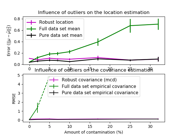
在這個例子中,我們比較了在受污染的高斯分布數據集上使用不同類型的位置估計和協方差估計時所產生的估計誤差:
整個數據集的均值和經驗協方差,一旦數據集中出現異常值就會分解。 穩健的MCD,它提供了一個較低的錯誤。 已知的好的觀測值的均值和經驗協方差。這可以被認為是一種“完美”的MCD估計,因此我們可以通過與這種情況進行比較來信任我們的實現。
參考
1 Johanna Hardin, David M Rocke. The distribution of robust distances. Journal of Computational and Graphical Statistics. December 1, 2005, 14(4): 928-946.
2 Zoubir A., Koivunen V., Chakhchoukh Y. and Muma M. (2012). Robust estimation in signal processing: A tutorial-style treatment of fundamental concepts. IEEE Signal Processing Magazine 29(4), 61-80.
3 P. J. Rousseeuw. Least median of squares regression. Journal of American Statistical Ass., 79:871, 1984
print(__doc__)

import numpy as np
import matplotlib.pyplot as plt
import matplotlib.font_manager

from sklearn.covariance import EmpiricalCovariance, MinCovDet

# example settings
n_samples = 80
n_features = 5
repeat = 10

range_n_outliers = np.concatenate(
    (np.linspace(0, n_samples / 8, 5),
     np.linspace(n_samples / 8, n_samples / 2, 5)[1:-1])).astype(np.int)

# definition of arrays to store results
err_loc_mcd = np.zeros((range_n_outliers.size, repeat))
err_cov_mcd = np.zeros((range_n_outliers.size, repeat))
err_loc_emp_full = np.zeros((range_n_outliers.size, repeat))
err_cov_emp_full = np.zeros((range_n_outliers.size, repeat))
err_loc_emp_pure = np.zeros((range_n_outliers.size, repeat))
err_cov_emp_pure = np.zeros((range_n_outliers.size, repeat))

# computation
for i, n_outliers in enumerate(range_n_outliers):
    for j in range(repeat):

        rng = np.random.RandomState(i * j)

        # generate data
        X = rng.randn(n_samples, n_features)
        # add some outliers
        outliers_index = rng.permutation(n_samples)[:n_outliers]
        outliers_offset = 10. * \
            (np.random.randint(2, size=(n_outliers, n_features)) - 0.5)
        X[outliers_index] += outliers_offset
        inliers_mask = np.ones(n_samples).astype(bool)
        inliers_mask[outliers_index] = False

        # fit a Minimum Covariance Determinant (MCD) robust estimator to data
        mcd = MinCovDet().fit(X)
        # compare raw robust estimates with the true location and covariance
        err_loc_mcd[i, j] = np.sum(mcd.location_ ** 2)
        err_cov_mcd[i, j] = mcd.error_norm(np.eye(n_features))

        # compare estimators learned from the full data set with true
        # parameters
        err_loc_emp_full[i, j] = np.sum(X.mean(0) ** 2)
        err_cov_emp_full[i, j] = EmpiricalCovariance().fit(X).error_norm(
            np.eye(n_features))

        # compare with an empirical covariance learned from a pure data set
        # (i.e. "perfect" mcd)
        pure_X = X[inliers_mask]
        pure_location = pure_X.mean(0)
        pure_emp_cov = EmpiricalCovariance().fit(pure_X)
        err_loc_emp_pure[i, j] = np.sum(pure_location ** 2)
        err_cov_emp_pure[i, j] = pure_emp_cov.error_norm(np.eye(n_features))

# Display results
font_prop = matplotlib.font_manager.FontProperties(size=11)
plt.subplot(2, 1, 1)
lw = 2
plt.errorbar(range_n_outliers, err_loc_mcd.mean(1),
             yerr=err_loc_mcd.std(1) / np.sqrt(repeat),
             label="Robust location", lw=lw, color='m')
plt.errorbar(range_n_outliers, err_loc_emp_full.mean(1),
             yerr=err_loc_emp_full.std(1) / np.sqrt(repeat),
             label="Full data set mean", lw=lw, color='green')
plt.errorbar(range_n_outliers, err_loc_emp_pure.mean(1),
             yerr=err_loc_emp_pure.std(1) / np.sqrt(repeat),
             label="Pure data set mean", lw=lw, color='black')
plt.title("Influence of outliers on the location estimation")
plt.ylabel(r"Error ($||\mu - \hat{\mu}||_2^2$)")
plt.legend(loc="upper left", prop=font_prop)

plt.subplot(2, 1, 2)
x_size = range_n_outliers.size
plt.errorbar(range_n_outliers, err_cov_mcd.mean(1),
             yerr=err_cov_mcd.std(1),
             label="Robust covariance (mcd)", color='m')
plt.errorbar(range_n_outliers[:(x_size // 5 + 1)],
             err_cov_emp_full.mean(1)[:(x_size // 5 + 1)],
             yerr=err_cov_emp_full.std(1)[:(x_size // 5 + 1)],
             label="Full data set empirical covariance", color='green')
plt.plot(range_n_outliers[(x_size // 5):(x_size // 2 - 1)],
         err_cov_emp_full.mean(1)[(x_size // 5):(x_size // 2 - 1)],
         color='green', ls='--')
plt.errorbar(range_n_outliers, err_cov_emp_pure.mean(1),
             yerr=err_cov_emp_pure.std(1),
             label="Pure data set empirical covariance", color='black')
plt.title("Influence of outliers on the covariance estimation")
plt.xlabel("Amount of contamination (%)")
plt.ylabel("RMSE")
plt.legend(loc="upper center", prop=font_prop)

plt.show()
腳本的總運行時間:(0分3.170秒)
Download Python source code:plot_robust_vs_empirical_covariance.py
Download Jupyter notebook:plot_robust_vs_empirical_covariance.ipynb