基于完全隨機樹的哈希特征變換?

RandomTreesEmbedding 提供了一種將數據映射到非常高維、稀疏表示的方法，這可能有利于分類。該映射是完全無監督和非常有效的。

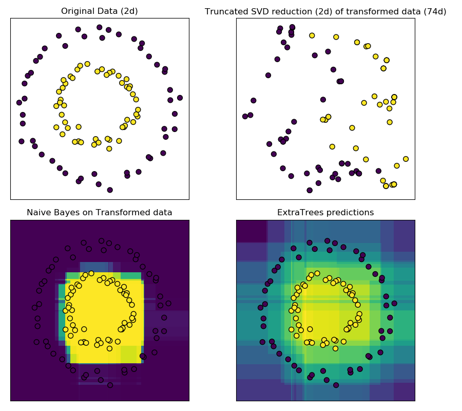
這個例子可視化了由幾個樹給出的分區，并展示了轉換也可以用于非線性維數約簡或非線性分類。

相鄰的點通常共享一棵樹的同一片葉子，因此他們的哈希表示共享一個大區域。這樣就可以將兩個同心圓簡單分離， 主要是基于轉換后數據的主成分， 使用帶約束的SVD。

在高維空間中，線性分類器往往具有很好的精度。對于稀疏二進制數據，bernoulliNB特別適合。下面一行將比較從BernoulliNB在轉換后數據集上訓練得到的決策邊界與使用極端隨機樹森林在原始數據集上訓練得到的決策邊界進行比較。

import numpy as np
import matplotlib.pyplot as plt

from sklearn.datasets import make_circles
from sklearn.ensemble import RandomTreesEmbedding, ExtraTreesClassifier
from sklearn.decomposition import TruncatedSVD
from sklearn.naive_bayes import BernoulliNB

# make a synthetic dataset
X, y = make_circles(factor=0.5, random_state=0, noise=0.05)

# use RandomTreesEmbedding to transform data
hasher = RandomTreesEmbedding(n_estimators=10, random_state=0, max_depth=3)
X_transformed = hasher.fit_transform(X)

# Visualize result after dimensionality reduction using truncated SVD
svd = TruncatedSVD(n_components=2)
X_reduced = svd.fit_transform(X_transformed)

# Learn a Naive Bayes classifier on the transformed data
nb = BernoulliNB()
nb.fit(X_transformed, y)


# Learn an ExtraTreesClassifier for comparison
trees = ExtraTreesClassifier(max_depth=3, n_estimators=10, random_state=0)
trees.fit(X, y)


# scatter plot of original and reduced data
fig = plt.figure(figsize=(9, 8))

ax = plt.subplot(221)
ax.scatter(X[:, 0], X[:, 1], c=y, s=50, edgecolor='k')
ax.set_title("Original Data (2d)")
ax.set_xticks(())
ax.set_yticks(())

ax = plt.subplot(222)
ax.scatter(X_reduced[:, 0], X_reduced[:, 1], c=y, s=50, edgecolor='k')
ax.set_title("Truncated SVD reduction (2d) of transformed data (%dd)" %
             X_transformed.shape[1])
ax.set_xticks(())
ax.set_yticks(())

# Plot the decision in original space. For that, we will assign a color
# to each point in the mesh [x_min, x_max]x[y_min, y_max].
h = .01
x_min, x_max = X[:, 0].min() - .5, X[:, 0].max() + .5
y_min, y_max = X[:, 1].min() - .5, X[:, 1].max() + .5
xx, yy = np.meshgrid(np.arange(x_min, x_max, h), np.arange(y_min, y_max, h))

# transform grid using RandomTreesEmbedding
transformed_grid = hasher.transform(np.c_[xx.ravel(), yy.ravel()])
y_grid_pred = nb.predict_proba(transformed_grid)[:, 1]

ax = plt.subplot(223)
ax.set_title("Naive Bayes on Transformed data")
ax.pcolormesh(xx, yy, y_grid_pred.reshape(xx.shape))
ax.scatter(X[:, 0], X[:, 1], c=y, s=50, edgecolor='k')
ax.set_ylim(-1.4, 1.4)
ax.set_xlim(-1.4, 1.4)
ax.set_xticks(())
ax.set_yticks(())

# transform grid using ExtraTreesClassifier
y_grid_pred = trees.predict_proba(np.c_[xx.ravel(), yy.ravel()])[:, 1]

ax = plt.subplot(224)
ax.set_title("ExtraTrees predictions")
ax.pcolormesh(xx, yy, y_grid_pred.reshape(xx.shape))
ax.scatter(X[:, 0], X[:, 1], c=y, s=50, edgecolor='k')
ax.set_ylim(-1.4, 1.4)
ax.set_xlim(-1.4, 1.4)
ax.set_xticks(())
ax.set_yticks(())

plt.tight_layout()
plt.show()

腳本的總運行時間：(0分0.437秒)

Download Python source code: plot_random_forest_embedding.py

Download Jupyter notebook:plot_random_forest_embedding.ipynb