單個估計器 vs bagging:偏差-方差分解?
此示例說明并比較了單個估計器的期望均方誤差與bagging 集成的偏差-方差分解。
在回歸中,估計器的期望均方誤差可以用偏差、方差和噪聲來分解。在回歸問題的平均數據集上,偏差項度量了估計器的預測與最優的可能的估計器的預測之間的不同的平均差異, 對問題而言(即Bayes模型)。方差項度量了對于問題而言,當擬合不同的實例LS的時候, 估計器的預測的變化程度。
最后,噪聲度量誤差的不可約部分,這是由于數據的變異性。
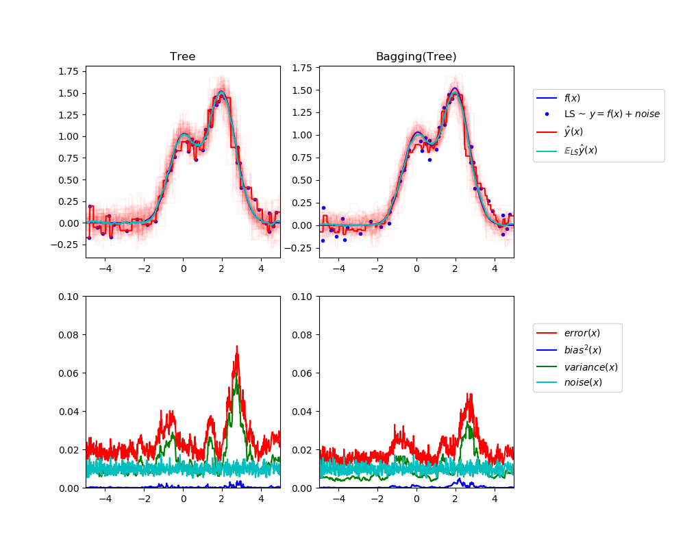
左上角的圖說明了一維回歸問題, 在玩具的隨機數據集LS(藍點)上訓練的單個決策樹的預測(以暗紅色表示)。它還說明了在其他隨機繪制實例LS上訓練的其他單個決策樹的預測(以淡紅色表示)。顯而易見地,這里的方差項對應于單個估計器的預測光束的寬度(以亮紅色表示)。方差越大,x對訓練集中微小變化的預測就越敏感。偏差項對應于估計器(青色)的平均預測值與最佳模型(深藍色)之間的差異。在這個問題上,我們可以觀察到偏差很小(藍曲線和青色曲線都很接近),而方差很大(紅色光束比較寬)。
左下角圖描繪了單個決策樹的期望均方誤差的點態分解。它證實了偏差項(藍色)是低的,而方差是大的(綠色)。它還說明了誤差的噪聲部分,如預期的,似乎是恒定的,在0.01左右。
右邊的圖對應是一樣的,但使用的bagging集成的一組決策樹。在這兩個圖中,我們可以觀察到偏差項比以前的情況要大。在右上角圖中,平均預測值(青色)與最佳模型之間的差異較大(例如,注意x=2附近的偏移量)。在右下角圖中,偏置曲線也略高于左下角圖。然而,就方差而言,預測束較窄,表明方差較小。事實上,正如右下角的數字所證實的,方差項(綠色)比單個決策樹的方差項要低。總的來說,偏差-方差分解不再是相同的。這種折衷更適合于bagging:在數據集的副本上平均幾個決策樹的結果會略微增加偏差項,但允許更大程度地減少方差,從而導致整體均方誤差較低(比較下圖中的紅色曲線)。腳本輸出也證實了這種直覺。bagging的總誤差小于單棵決策樹的總誤差,這種差異確實主要是由于方差的減小所致。
關于偏差-方差分解的更多細節,見[1]中的7.3章節。
參考
1 T. Hastie, R. Tibshirani and J. Friedman, “Elements of Statistical Learning”, Springer, 2009.
Tree: 0.0255 (error) = 0.0003 (bias^2)  + 0.0152 (var) + 0.0098 (noise)
Bagging(Tree): 0.0196 (error) = 0.0004 (bias^2)  + 0.0092 (var) + 0.0098 (noise)
print(__doc__)

# Author: Gilles Louppe <g.louppe@gmail.com>
# License: BSD 3 clause

import numpy as np
import matplotlib.pyplot as plt

from sklearn.ensemble import BaggingRegressor
from sklearn.tree import DecisionTreeRegressor

# Settings
n_repeat = 50       # Number of iterations for computing expectations
n_train = 50        # Size of the training set
n_test = 1000       # Size of the test set
noise = 0.1         # Standard deviation of the noise
np.random.seed(0)

# Change this for exploring the bias-variance decomposition of other
# estimators. This should work well for estimators with high variance (e.g.,
# decision trees or KNN), but poorly for estimators with low variance (e.g.,
# linear models).
estimators = [("Tree", DecisionTreeRegressor()),
              ("Bagging(Tree)", BaggingRegressor(DecisionTreeRegressor()))]

n_estimators = len(estimators)


# Generate data
def f(x):
    x = x.ravel()

    return np.exp(-x ** 2) + 1.5 * np.exp(-(x - 2) ** 2)


def generate(n_samples, noise, n_repeat=1):
    X = np.random.rand(n_samples) * 10 - 5
    X = np.sort(X)

    if n_repeat == 1:
        y = f(X) + np.random.normal(0.0, noise, n_samples)
    else:
        y = np.zeros((n_samples, n_repeat))

        for i in range(n_repeat):
            y[:, i] = f(X) + np.random.normal(0.0, noise, n_samples)

    X = X.reshape((n_samples, 1))

    return X, y


X_train = []
y_train = []

for i in range(n_repeat):
    X, y = generate(n_samples=n_train, noise=noise)
    X_train.append(X)
    y_train.append(y)

X_test, y_test = generate(n_samples=n_test, noise=noise, n_repeat=n_repeat)

plt.figure(figsize=(10, 8))

# Loop over estimators to compare
for n, (name, estimator) in enumerate(estimators):
    # Compute predictions
    y_predict = np.zeros((n_test, n_repeat))

    for i in range(n_repeat):
        estimator.fit(X_train[i], y_train[i])
        y_predict[:, i] = estimator.predict(X_test)

    # Bias^2 + Variance + Noise decomposition of the mean squared error
    y_error = np.zeros(n_test)

    for i in range(n_repeat):
        for j in range(n_repeat):
            y_error += (y_test[:, j] - y_predict[:, i]) ** 2

    y_error /= (n_repeat * n_repeat)

    y_noise = np.var(y_test, axis=1)
    y_bias = (f(X_test) - np.mean(y_predict, axis=1)) ** 2
    y_var = np.var(y_predict, axis=1)

    print("{0}: {1:.4f} (error) = {2:.4f} (bias^2) "
          " + {3:.4f} (var) + {4:.4f} (noise)".format(name,
                                                      np.mean(y_error),
                                                      np.mean(y_bias),
                                                      np.mean(y_var),
                                                      np.mean(y_noise)))

    # Plot figures
    plt.subplot(2, n_estimators, n + 1)
    plt.plot(X_test, f(X_test), "b", label="$f(x)$")
    plt.plot(X_train[0], y_train[0], ".b", label="LS ~ $y = f(x)+noise$")

    for i in range(n_repeat):
        if i == 0:
            plt.plot(X_test, y_predict[:, i], "r", label=r"$\^y(x)$")
        else:
            plt.plot(X_test, y_predict[:, i], "r", alpha=0.05)

    plt.plot(X_test, np.mean(y_predict, axis=1), "c",
             label=r"$\mathbb{E}_{LS} \^y(x)$")

    plt.xlim([-5, 5])
    plt.title(name)

    if n == n_estimators - 1:
        plt.legend(loc=(1.1, .5))

    plt.subplot(2, n_estimators, n_estimators + n + 1)
    plt.plot(X_test, y_error, "r", label="$error(x)$")
    plt.plot(X_test, y_bias, "b", label="$bias^2(x)$"),
    plt.plot(X_test, y_var, "g", label="$variance(x)$"),
    plt.plot(X_test, y_noise, "c", label="$noise(x)$")

    plt.xlim([-5, 5])
    plt.ylim([0, 0.1])

    if n == n_estimators - 1:

        plt.legend(loc=(1.1, .5))

plt.subplots_adjust(right=.75)
plt.show()
腳本的總運行時間:(0分1.587秒)