核嶺回歸與高斯過程回歸的比較?
核嶺回歸(KRR)和高斯過程回歸(GPR)都是通過內部使用“核技巧”來學習目標函數的。KRR在相應的核催生的空間中學習一個線性函數,該函數對應于原始空間中的一個非線性函數。線性函數的選擇是基于帶嶺正則的軍方誤差損失。GPR使用核來定義目標函數的先驗分布的協方差,并使用觀測到的訓練數據來定義似然函數。基于Bayes定理,定義了目標函數上的(高斯)后驗分布,其均值用于預測。
一個主要的區別是,GPR可以基于邊際似然函數的梯度上升來選擇核的超參數,而KRR則需要對交叉驗證的損失函數(均方誤差損失)執行網格搜索。另一個不同之處是,GPR學習目標函數的生成概率模型,因此可以提供有意義的置信區間和后驗樣本以及預測,而KRR只提供預測。
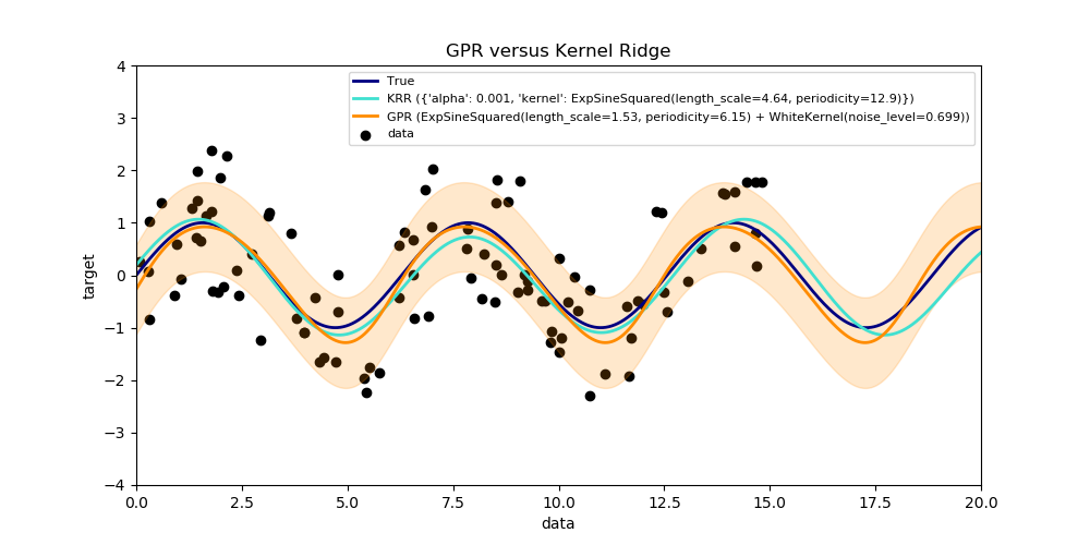
此示例說明了人工數據集上的這兩種方法,該數據集由一個正弦目標函數和強噪聲組成。圖中比較了KRR和GPR學習到模型, 基于的是ExpSineSquared核, 這個核適用于學習周期函數。核的超參數控制核的光滑性(L)和周期性(P)。此外,數據的噪聲水平是由GPR通過內核中附加的WhiteKernel成分和KRR的正則化參數α顯式地學習的。
此圖顯示,這兩種方法都學習了目標函數的合理模型。GPR正確地識別出函數的周期約為2*pi(6.28),而KRR選擇的雙倍的周期為4*pi。此外, GPR為預測提供了合理的置信界限, 但是KRR沒有不能獲取。這兩種方法的一個主要區別是擬合和預測所需的時間:雖然擬合KRR在原則上是快速的,但網格搜索的超參數優化規模與超參數的數量成指數關系(“維數詛咒”)。在GPR中基于梯度的參數優化不會遭受這種指數尺度的影響, 因此在這個具有三維超參數空間的例子中,速度要快得多。然而,預測的時間是相似的,GPR產生預測分布的方差要比僅僅預測平均值花費的時間要長得多。
Time for KRR fitting: 4.593
Time for GPR fitting: 0.105
Time for KRR prediction: 0.054
Time for GPR prediction: 0.078
Time for GPR prediction with standard-deviation: 0.084
print(__doc__)

# Authors: Jan Hendrik Metzen <jhm@informatik.uni-bremen.de>
# License: BSD 3 clause


import time

import numpy as np

import matplotlib.pyplot as plt

from sklearn.kernel_ridge import KernelRidge
from sklearn.model_selection import GridSearchCV
from sklearn.gaussian_process import GaussianProcessRegressor
from sklearn.gaussian_process.kernels import WhiteKernel, ExpSineSquared

rng = np.random.RandomState(0)

# Generate sample data
X = 15 * rng.rand(100, 1)
y = np.sin(X).ravel()
y += 3 * (0.5 - rng.rand(X.shape[0]))  # add noise

# Fit KernelRidge with parameter selection based on 5-fold cross validation
param_grid = {"alpha": [1e0, 1e-1, 1e-2, 1e-3],
              "kernel": [ExpSineSquared(l, p)
                         for l in np.logspace(-2, 2, 10)
                         for p in np.logspace(0, 2, 10)]}
kr = GridSearchCV(KernelRidge(), param_grid=param_grid)
stime = time.time()
kr.fit(X, y)
print("Time for KRR fitting: %.3f" % (time.time() - stime))

gp_kernel = ExpSineSquared(1.0, 5.0, periodicity_bounds=(1e-2, 1e1)) \
    + WhiteKernel(1e-1)
gpr = GaussianProcessRegressor(kernel=gp_kernel)
stime = time.time()
gpr.fit(X, y)
print("Time for GPR fitting: %.3f" % (time.time() - stime))

# Predict using kernel ridge
X_plot = np.linspace(0, 20, 10000)[:, None]
stime = time.time()
y_kr = kr.predict(X_plot)
print("Time for KRR prediction: %.3f" % (time.time() - stime))

# Predict using gaussian process regressor
stime = time.time()
y_gpr = gpr.predict(X_plot, return_std=False)
print("Time for GPR prediction: %.3f" % (time.time() - stime))

stime = time.time()
y_gpr, y_std = gpr.predict(X_plot, return_std=True)
print("Time for GPR prediction with standard-deviation: %.3f"
      % (time.time() - stime))

# Plot results
plt.figure(figsize=(10, 5))
lw = 2
plt.scatter(X, y, c='k', label='data')
plt.plot(X_plot, np.sin(X_plot), color='navy', lw=lw, label='True')
plt.plot(X_plot, y_kr, color='turquoise', lw=lw,
         label='KRR (%s)' % kr.best_params_)
plt.plot(X_plot, y_gpr, color='darkorange', lw=lw,
         label='GPR (%s)' % gpr.kernel_)
plt.fill_between(X_plot[:, 0], y_gpr - y_std, y_gpr + y_std, color='darkorange',
                 alpha=0.2)
plt.xlabel('data')
plt.ylabel('target')
plt.xlim(0, 20)
plt.ylim(-4, 4)
plt.title('GPR versus Kernel Ridge')
plt.legend(loc="best",  scatterpoints=1, prop={'size': 8})
plt.show()
腳本的總運行時間:(0分5.065秒)