繪制L2正則化函數的嶺系數圖?
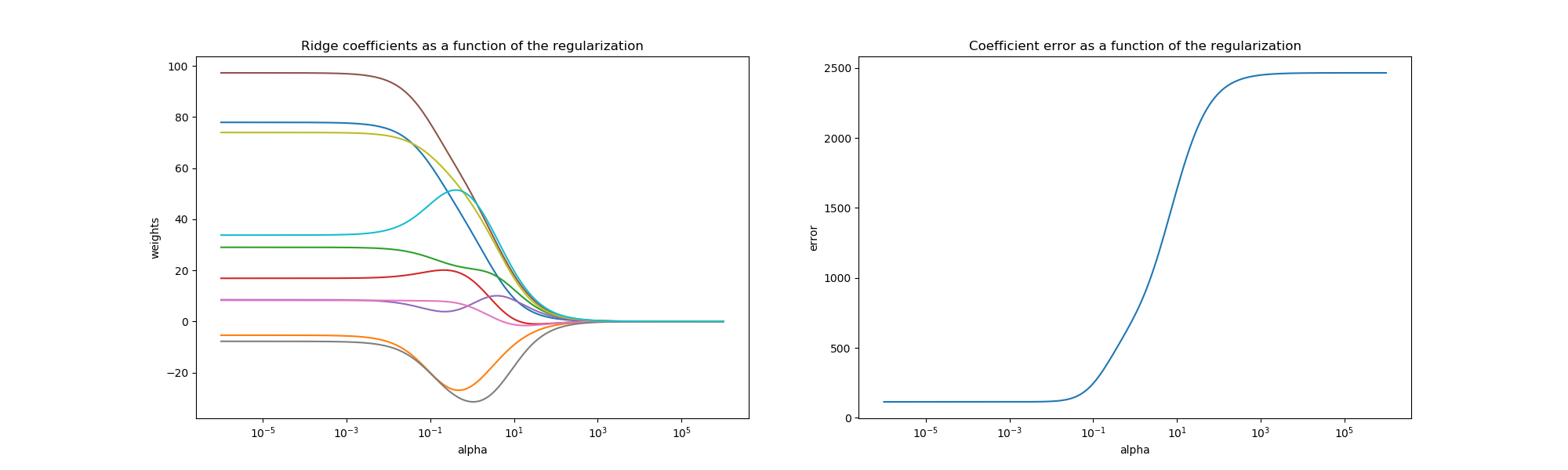
嶺回歸是在這個例子中使用的估計器。左圖中的每一種顏色表示系數向量的一個不同維度,表示為正則化參數的函數。右圖表顯示了解決方案的有多精確。此示例說明如何通過嶺回歸找到定義良好的解,以及正則化如何影響系數及其值。右邊的圖顯示了作為正則化函數的系數與估計與的差異是如何變化的。
在這個例子中,因變量Y被設為輸入特征的函數:y=X*w+c,系數向量w從正態分布隨機抽樣,而偏差項c被設置為常數。
當α趨于零時,嶺回歸發現的系數向隨機采樣向量w穩定。對于大 alpha(強正則化),系數較小(最終收斂于0),從而得到一個更簡單的有偏解。這些依賴關系可以在左邊的圖上觀察到。
右圖顯示了模型發現的系數與所選向量w之間的均方誤差,正則化程度較低的模型檢索到的精確系數(誤差等于0),強正則化模型增加了誤差。
請注意,在這個例子中,數據是無噪聲的,因此可以提取精確的系數。
# Author: Kornel Kielczewski -- <kornel.k@plusnet.pl>

print(__doc__)

import matplotlib.pyplot as plt
import numpy as np

from sklearn.datasets import make_regression
from sklearn.linear_model import Ridge
from sklearn.metrics import mean_squared_error

clf = Ridge()

X, y, w = make_regression(n_samples=10, n_features=10, coef=True,
                          random_state=1, bias=3.5)

coefs = []
errors = []

alphas = np.logspace(-6, 6, 200)

# Train the model with different regularisation strengths
for a in alphas:
    clf.set_params(alpha=a)
    clf.fit(X, y)
    coefs.append(clf.coef_)
    errors.append(mean_squared_error(clf.coef_, w))

# Display results
plt.figure(figsize=(20, 6))

plt.subplot(121)
ax = plt.gca()
ax.plot(alphas, coefs)
ax.set_xscale('log')
plt.xlabel('alpha')
plt.ylabel('weights')
plt.title('Ridge coefficients as a function of the regularization')
plt.axis('tight')

plt.subplot(122)
ax = plt.gca()
ax.plot(alphas, errors)
ax.set_xscale('log')
plt.xlabel('alpha')
plt.ylabel('error')
plt.title('Coefficient error as a function of the regularization')
plt.axis('tight')

plt.show()
腳本的總運行時間:(0分0.376秒)