線性回歸實例?
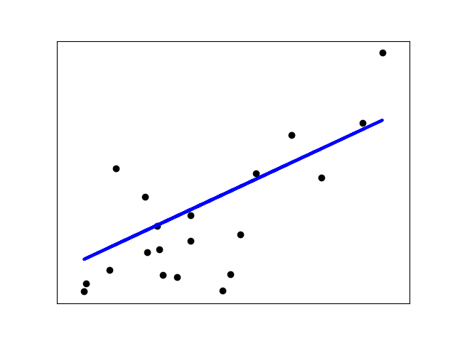
此示例僅使用 diabetes數據集的第一個特征,以說明此回歸技術的二維繪圖。在圖中可以看到直線,顯示線性回歸如何試圖繪制一條直線,使數據集中觀察到的響應與線性近似預測的響應之間的殘差平方和最小化。
計算了系數、殘差平方和及確定系數。
Coefficients:
 [938.23786125]
Mean squared error: 2548.07
Coefficient of determination: 0.47
print(__doc__)


# Code source: Jaques Grobler
# License: BSD 3 clause


import matplotlib.pyplot as plt
import numpy as np
from sklearn import datasets, linear_model
from sklearn.metrics import mean_squared_error, r2_score

# Load the diabetes dataset
diabetes_X, diabetes_y = datasets.load_diabetes(return_X_y=True)

# Use only one feature
diabetes_X = diabetes_X[:, np.newaxis, 2]

# Split the data into training/testing sets
diabetes_X_train = diabetes_X[:-20]
diabetes_X_test = diabetes_X[-20:]

# Split the targets into training/testing sets
diabetes_y_train = diabetes_y[:-20]
diabetes_y_test = diabetes_y[-20:]

# Create linear regression object
regr = linear_model.LinearRegression()

# Train the model using the training sets
regr.fit(diabetes_X_train, diabetes_y_train)

# Make predictions using the testing set
diabetes_y_pred = regr.predict(diabetes_X_test)

# The coefficients
print('Coefficients: \n', regr.coef_)
# The mean squared error
print('Mean squared error: %.2f'
      % mean_squared_error(diabetes_y_test, diabetes_y_pred))
# The coefficient of determination: 1 is perfect prediction
print('Coefficient of determination: %.2f'
      % r2_score(diabetes_y_test, diabetes_y_pred))

# Plot outputs
plt.scatter(diabetes_X_test, diabetes_y_test,  color='black')
plt.plot(diabetes_X_test, diabetes_y_pred, color='blue', linewidth=3)

plt.xticks(())
plt.yticks(())

plt.show()
腳本的總運行時間:(0分0.048秒)