Theil-Sen回歸?
在合成數據集上計算Theil-Sen回歸。
有關回歸器的更多信息,請參見 Theil-Sen estimator: generalized-median-based estimator。
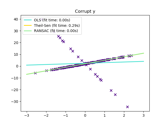
與OLS(普通最小二乘)估計相比,Theil-Sen估計對異常值具有較強的魯棒性。在簡單線性回歸的情況下,它的崩潰點約為29.3%,這意味著它在二維情況下可以容忍任意損壞的數據(異常值)占比高達29.3%。
模型的估計是通過計算p子樣本點的所有可能組合的子種群的斜率和截取來完成的。如果擬合了截距,則p必須大于或等于n_features + 1。最后的斜率和截距定義為這些斜率和截距的空間中值。
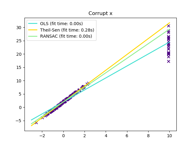
在某些情況下,Theil-Sen的性能優于 RANSAC,這也是一種很穩健的方法。這在下面的第二個例子中得到了說明,其中帶異常值x軸擾動的RANSAC。調整RANSAC的 residual_threshold 參數可以彌補這一點,但是一般來說,需要對數據和異常值的性質有一個先驗的了解。由于Theil-Sen計算的復雜性,建議只在樣本數量和特征方面的小問題上使用它。對于較大的問題, max_subpopulation 參數將p子樣本點的所有可能組合的大小限制為隨機選擇的子集,因此也限制了運行時。因此,Theil-Sen適用于較大的問題,其缺點是失去了它的一些數學性質,因為它是在隨機子集上工作的。
# Author: Florian Wilhelm -- <florian.wilhelm@gmail.com>
# License: BSD 3 clause

import time
import numpy as np
import matplotlib.pyplot as plt
from sklearn.linear_model import LinearRegression, TheilSenRegressor
from sklearn.linear_model import RANSACRegressor

print(__doc__)

estimators = [('OLS', LinearRegression()),
              ('Theil-Sen', TheilSenRegressor(random_state=42)),
              ('RANSAC', RANSACRegressor(random_state=42)), ]
colors = {'OLS': 'turquoise', 'Theil-Sen': 'gold', 'RANSAC': 'lightgreen'}
lw = 2

# #############################################################################
# Outliers only in the y direction

np.random.seed(0)
n_samples = 200
# Linear model y = 3*x + N(2, 0.1**2)
x = np.random.randn(n_samples)
w = 3.
c = 2.
noise = 0.1 * np.random.randn(n_samples)
y = w * x + c + noise
# 10% outliers
y[-20:] += -20 * x[-20:]
X = x[:, np.newaxis]

plt.scatter(x, y, color='indigo', marker='x', s=40)
line_x = np.array([-3, 3])
for name, estimator in estimators:
    t0 = time.time()
    estimator.fit(X, y)
    elapsed_time = time.time() - t0
    y_pred = estimator.predict(line_x.reshape(2, 1))
    plt.plot(line_x, y_pred, color=colors[name], linewidth=lw,
             label='%s (fit time: %.2fs)' % (name, elapsed_time))

plt.axis('tight')
plt.legend(loc='upper left')
plt.title("Corrupt y")

# #############################################################################
# Outliers in the X direction

np.random.seed(0)
# Linear model y = 3*x + N(2, 0.1**2)
x = np.random.randn(n_samples)
noise = 0.1 * np.random.randn(n_samples)
y = 3 * x + 2 + noise
# 10% outliers
x[-20:] = 9.9
y[-20:] += 22
X = x[:, np.newaxis]

plt.figure()
plt.scatter(x, y, color='indigo', marker='x', s=40)

line_x = np.array([-3, 10])
for name, estimator in estimators:
    t0 = time.time()
    estimator.fit(X, y)
    elapsed_time = time.time() - t0
    y_pred = estimator.predict(line_x.reshape(2, 1))
    plt.plot(line_x, y_pred, color=colors[name], linewidth=lw,
             label='%s (fit time: %.2fs)' % (name, elapsed_time))

plt.axis('tight')
plt.legend(loc='upper left')
plt.title("Corrupt x")
plt.show()
腳本的總運行時間:(0分0.749秒)。