貝葉斯嶺回歸?
在合成數據集上計算貝葉斯嶺回歸。
有關回歸的更多信息,請參見貝葉斯嶺回歸。
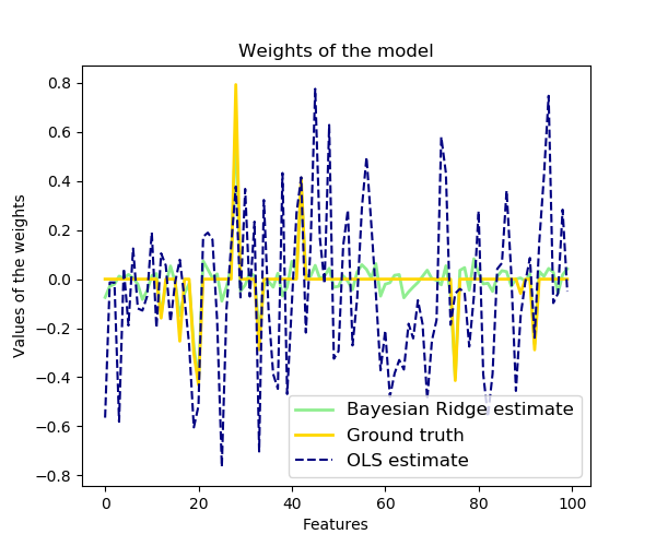
與普通最小二乘估計相比,系數權值略有移向零,從而使其穩定。
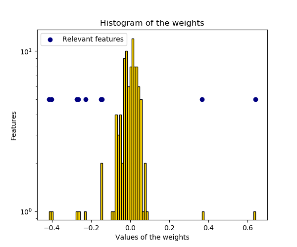
由于權值的先驗是高斯先驗,估計權值的直方圖是高斯的。
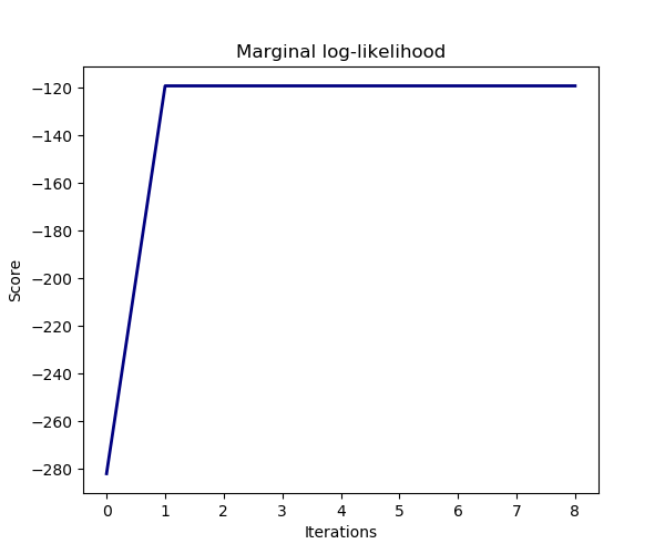
模型的估計是通過迭代最大化觀測的邊際對數似然來實現的。
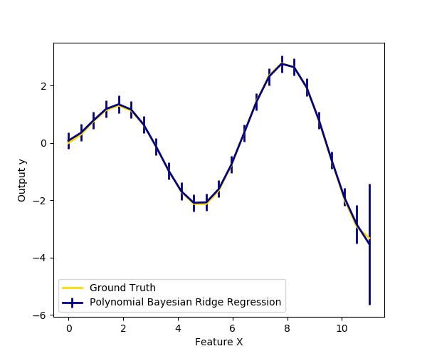
我們還用多項式特征擴展法繪制了一維回歸的貝葉斯嶺回歸的預測和不確定性圖。請注意,在右邊的圖中不確定性開始上升這是因為這些測試樣本超出了訓練樣本的范圍。
print(__doc__)

import numpy as np
import matplotlib.pyplot as plt
from scipy import stats

from sklearn.linear_model import BayesianRidge, LinearRegression

# #############################################################################
# Generating simulated data with Gaussian weights
np.random.seed(0)
n_samples, n_features = 100, 100
X = np.random.randn(n_samples, n_features)  # Create Gaussian data
# Create weights with a precision lambda_ of 4.
lambda_ = 4.
w = np.zeros(n_features)
# Only keep 10 weights of interest
relevant_features = np.random.randint(0, n_features, 10)
for i in relevant_features:
    w[i] = stats.norm.rvs(loc=0, scale=1. / np.sqrt(lambda_))
# Create noise with a precision alpha of 50.
alpha_ = 50.
noise = stats.norm.rvs(loc=0, scale=1. / np.sqrt(alpha_), size=n_samples)
# Create the target
y = np.dot(X, w) + noise

# #############################################################################
# Fit the Bayesian Ridge Regression and an OLS for comparison
clf = BayesianRidge(compute_score=True)
clf.fit(X, y)

ols = LinearRegression()
ols.fit(X, y)

# #############################################################################
# Plot true weights, estimated weights, histogram of the weights, and
# predictions with standard deviations
lw = 2
plt.figure(figsize=(6, 5))
plt.title("Weights of the model")
plt.plot(clf.coef_, color='lightgreen', linewidth=lw,
         label="Bayesian Ridge estimate")
plt.plot(w, color='gold', linewidth=lw, label="Ground truth")
plt.plot(ols.coef_, color='navy', linestyle='--', label="OLS estimate")
plt.xlabel("Features")
plt.ylabel("Values of the weights")
plt.legend(loc="best", prop=dict(size=12))

plt.figure(figsize=(6, 5))
plt.title("Histogram of the weights")
plt.hist(clf.coef_, bins=n_features, color='gold', log=True,
         edgecolor='black')
plt.scatter(clf.coef_[relevant_features], np.full(len(relevant_features), 5.),
            color='navy', label="Relevant features")
plt.ylabel("Features")
plt.xlabel("Values of the weights")
plt.legend(loc="upper left")

plt.figure(figsize=(6, 5))
plt.title("Marginal log-likelihood")
plt.plot(clf.scores_, color='navy', linewidth=lw)
plt.ylabel("Score")
plt.xlabel("Iterations")


# Plotting some predictions for polynomial regression
def f(x, noise_amount):
    y = np.sqrt(x) * np.sin(x)
    noise = np.random.normal(0, 1, len(x))
    return y + noise_amount * noise


degree = 10
X = np.linspace(0, 10, 100)
y = f(X, noise_amount=0.1)
clf_poly = BayesianRidge()
clf_poly.fit(np.vander(X, degree), y)

X_plot = np.linspace(0, 11, 25)
y_plot = f(X_plot, noise_amount=0)
y_mean, y_std = clf_poly.predict(np.vander(X_plot, degree), return_std=True)
plt.figure(figsize=(6, 5))
plt.errorbar(X_plot, y_mean, y_std, color='navy',
             label="Polynomial Bayesian Ridge Regression", linewidth=lw)
plt.plot(X_plot, y_plot, color='gold', linewidth=lw,
         label="Ground Truth")
plt.ylabel("Output y")
plt.xlabel("Feature X")
plt.legend(loc="lower left")
plt.show()
腳本的總運行時間:(0分0.500秒)