支持向量機的邊際?

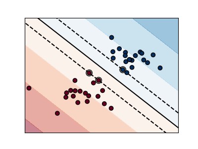
下圖顯示了參數C對分隔線的影響。 設置較大的C值相當于告訴我們的模型，我們對數據的分布沒有太大的信心，只會考慮更接近分隔線的點。

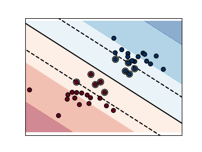
較小的C值包含更多/所有觀察值，從而可以使用該區域中的所有數據來計算邊距。

輸入：

print(__doc__)


# 源代碼: Ga?l Varoquaux
# 由Jaques Grobler編輯成文檔
# 執照: BSD 3 clause

import numpy as np
import matplotlib.pyplot as plt
from sklearn import svm

# 我們創建40個分離的點
np.random.seed(0)
X = np.r_[np.random.randn(20, 2) - [2, 2], np.random.randn(20, 2) + [2, 2]]
Y = [0] * 20 + [1] * 20

# 圖像的編號
fignum = 1

# 擬合模型
for name, penalty in (('unreg', 1), ('reg', 0.05)):

    clf = svm.SVC(kernel='linear', C=penalty)
    clf.fit(X, Y)

    # 得到分割超平面
    w = clf.coef_[0]
    a = -w[0] / w[1]
    xx = np.linspace(-5, 5)
    yy = a * xx - (clf.intercept_[0]) / w[1]

    # 繪制與穿過支持向量、與分割超平面平行的平行線（邊際：在垂直于超平面的方向上，平行線遠離超平面的距離）。二維距離垂直方向為sqrt（1 + a ^ 2）。
    margin = 1 / np.sqrt(np.sum(clf.coef_ ** 2))
    yy_down = yy - np.sqrt(1 + a ** 2) * margin
    yy_up = yy + np.sqrt(1 + a ** 2) * margin

    # 繪制直線，點和最接近平面的向量
    plt.figure(fignum, figsize=(4, 3))
    plt.clf()
    plt.plot(xx, yy, 'k-')
    plt.plot(xx, yy_down, 'k--')
    plt.plot(xx, yy_up, 'k--')

    plt.scatter(clf.support_vectors_[:, 0], clf.support_vectors_[:, 1], s=80,
                facecolors='none', zorder=10, edgecolors='k')
    plt.scatter(X[:, 0], X[:, 1], c=Y, zorder=10, cmap=plt.cm.Paired,
                edgecolors='k')

    plt.axis('tight')
    x_min = -4.8
    x_max = 4.2
    y_min = -6
    y_max = 6

    XX, YY = np.mgrid[x_min:x_max:200j, y_min:y_max:200j]
    Z = clf.predict(np.c_[XX.ravel(), YY.ravel()])

    # 將結果放入彩色圖像
    Z = Z.reshape(XX.shape)
    plt.figure(fignum, figsize=(4, 3))
    plt.pcolormesh(XX, YY, Z, cmap=plt.cm.Paired)

    plt.xlim(x_min, x_max)
    plt.ylim(y_min, y_max)

    plt.xticks(())
    plt.yticks(())
    fignum = fignum + 1

plt.show()

腳本的總運行時間：（0分鐘0.145秒）