二維數字嵌入上的各種凝聚聚類?
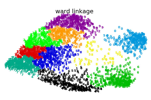
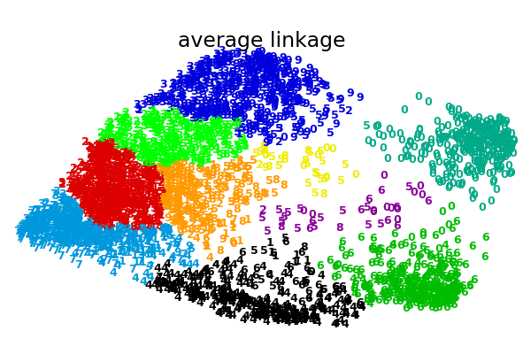
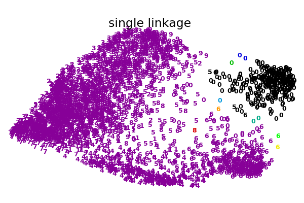
在數字數據集的2D嵌入上用于聚集聚類的各種鏈接選項的說明。
此示例的目標是直觀地顯示指標的行為,而不是為數字找到好的聚類。這就是為什么這個例子適用于2D嵌入。
這個例子向我們展示的是聚集性聚類的“rich getting richer”的行為,這種行為往往會造成不均勻的聚類大小。這種行為對于平均鏈接策略來說是非常明顯的,它最終產生了幾個單點簇,而在單個鏈接中,我們得到了一個單一的中心簇,所有其他的簇都是從邊緣的噪聲點中提取出來的。
Computing embedding
Done.
ward :  0.42s
average :       0.44s
complete :      0.42s
single :        0.10s
# Authors: Gael Varoquaux
# License: BSD 3 clause (C) INRIA 2014

print(__doc__)
from time import time

import numpy as np
from scipy import ndimage
from matplotlib import pyplot as plt

from sklearn import manifold, datasets

X, y = datasets.load_digits(return_X_y=True)
n_samples, n_features = X.shape

np.random.seed(0)

def nudge_images(X, y):
    # Having a larger dataset shows more clearly the behavior of the
    # methods, but we multiply the size of the dataset only by 2, as the
    # cost of the hierarchical clustering methods are strongly
    # super-linear in n_samples
    shift = lambda x: ndimage.shift(x.reshape((8, 8)),
                                  .3 * np.random.normal(size=2),
                                  mode='constant',
                                  ).ravel()
    X = np.concatenate([X, np.apply_along_axis(shift, 1, X)])
    Y = np.concatenate([y, y], axis=0)
    return X, Y


X, y = nudge_images(X, y)


#----------------------------------------------------------------------
# Visualize the clustering
def plot_clustering(X_red, labels, title=None):
    x_min, x_max = np.min(X_red, axis=0), np.max(X_red, axis=0)
    X_red = (X_red - x_min) / (x_max - x_min)

    plt.figure(figsize=(6, 4))
    for i in range(X_red.shape[0]):
        plt.text(X_red[i, 0], X_red[i, 1], str(y[i]),
                 color=plt.cm.nipy_spectral(labels[i] / 10.),
                 fontdict={'weight': 'bold', 'size': 9})

    plt.xticks([])
    plt.yticks([])
    if title is not None:
        plt.title(title, size=17)
    plt.axis('off')
    plt.tight_layout(rect=[0, 0.03, 1, 0.95])

#----------------------------------------------------------------------
# 2D embedding of the digits dataset
print("Computing embedding")
X_red = manifold.SpectralEmbedding(n_components=2).fit_transform(X)
print("Done.")

from sklearn.cluster import AgglomerativeClustering

for linkage in ('ward', 'average', 'complete', 'single'):
    clustering = AgglomerativeClustering(linkage=linkage, n_clusters=10)
    t0 = time()
    clustering.fit(X_red)
    print("%s :\t%.2fs" % (linkage, time() - t0))

    plot_clustering(X_red, clustering.labels_, "%s linkage" % linkage)


plt.show()
腳本的總運行時間:(0分32.660秒)