具有成本復雜度的后剪枝決策樹?
DecisionTreeClassifier 提供了一些參數,如 min_samples_leaf和max_depth,以防止樹過擬合。成本復雜度剪枝提供了另一個控制樹大小的選項。在 DecisionTreeClassifier中, 這種剪枝技術是通過成本復雜度參數ccp_alpha來參數化的。更大的ccp_alpha值增加被剪枝的節點數。這里我們只展示了 ccp_alpha對樹的正則化的影響,以及如何根據驗證分數來選擇ccp_alpha。
有關剪枝的詳細信息,請參見最小成本復雜度剪枝。
print(__doc__)
import matplotlib.pyplot as plt
from sklearn.model_selection import train_test_split
from sklearn.datasets import load_breast_cancer
from sklearn.tree import DecisionTreeClassifier
葉子的總不存度 VS 被剪枝樹的有效alphas
最小成本復雜度剪枝是遞歸地找到 “weakest link”的節點。 weakest link是一個通過有效的 alpha進行參數化的,其中最小的有效的alpha的節點首先被剪枝。
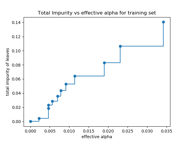
為了了解ccp_alpha的哪些值可能是合適的,scikit-learn提供了DecisionTreeClassifier.cost_complexity_pruning_path在修剪過程中每一步返回有效的alphas和相應的總葉子不存度。隨著alpha的增加,更多的樹被修剪,這增加了它的葉子的總不存度。
X, y = load_breast_cancer(return_X_y=True)
X_train, X_test, y_train, y_test = train_test_split(X, y, random_state=0)

clf = DecisionTreeClassifier(random_state=0)
path = clf.cost_complexity_pruning_path(X_train, y_train)
ccp_alphas, impurities = path.ccp_alphas, path.impurities
在下面的圖中,最大有效alpha值被刪除,因為它是只有一個節點的很普通的樹。
fig, ax = plt.subplots()
ax.plot(ccp_alphas[:-1], impurities[:-1], marker='o', drawstyle="steps-post")
ax.set_xlabel("effective alpha")
ax.set_ylabel("total impurity of leaves")
ax.set_title("Total Impurity vs effective alpha for training set")
Text(0.5, 1.0, 'Total Impurity vs effective alpha for training set')
接下來,我們使用有效的alphas來訓練決策樹。 ccp_alphas中的最后一個值是修剪整棵樹的alpha值,而樹clfs[-1]只有一個節點。
clfs = []
for ccp_alpha in ccp_alphas:
    clf = DecisionTreeClassifier(random_state=0, ccp_alpha=ccp_alpha)
    clf.fit(X_train, y_train)
    clfs.append(clf)
print("Number of nodes in the last tree is: {} with ccp_alpha: {}".format(
      clfs[-1].tree_.node_count, ccp_alphas[-1]))
Number of nodes in the last tree is: 1 with ccp_alpha: 0.3272984419327777
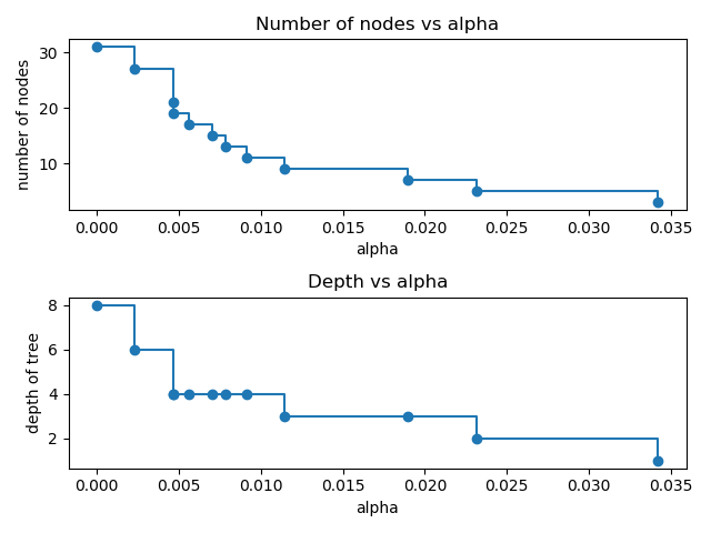
對于本例的其余部分,我們移除 clfs 和ccp_alphas中的最后一個元素,因為它是只有一個節點的很普通的樹。在這里,我們證明了節點數和樹的深度隨著 alpha 的增加而減少。
clfs = clfs[:-1]
ccp_alphas = ccp_alphas[:-1]

node_counts = [clf.tree_.node_count for clf in clfs]
depth = [clf.tree_.max_depth for clf in clfs]
fig, ax = plt.subplots(2, 1)
ax[0].plot(ccp_alphas, node_counts, marker='o', drawstyle="steps-post")
ax[0].set_xlabel("alpha")
ax[0].set_ylabel("number of nodes")
ax[0].set_title("Number of nodes vs alpha")
ax[1].plot(ccp_alphas, depth, marker='o', drawstyle="steps-post")
ax[1].set_xlabel("alpha")
ax[1].set_ylabel("depth of tree")
ax[1].set_title("Depth vs alpha")
fig.tight_layout()
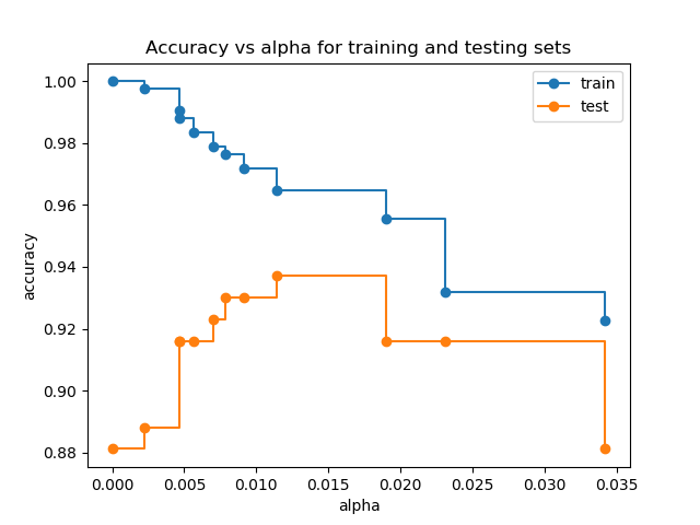
訓練和測試集的準確率 vs alpha
當 ccp_alpha 設置為0, 并保留DecisionTreeClassifier的其他默認參數時, 樹就過擬合了,使訓練的準確率達到100%,測試的準確率達到88%。隨著alpha的增加,更多的樹被剪枝,從而創建了一個泛化更好的決策樹。在本例中,設置 ccp_alpha=0.015可以最大限度地提高測試的準確率。
train_scores = [clf.score(X_train, y_train) for clf in clfs]
test_scores = [clf.score(X_test, y_test) for clf in clfs]

fig, ax = plt.subplots()
ax.set_xlabel("alpha")
ax.set_ylabel("accuracy")
ax.set_title("Accuracy vs alpha for training and testing sets")
ax.plot(ccp_alphas, train_scores, marker='o', label="train",
        drawstyle="steps-post")
ax.plot(ccp_alphas, test_scores, marker='o', label="test",
        drawstyle="steps-post")
ax.legend()
plt.show()
 腳本的總運行時間:(0分0.427秒)
Download Python source code: plot_cost_complexity_pruning.py
Download Jupyter notebook:plot_cost_complexity_pruning.ipynb