分類器校準的比較?

舉例說明分類器預測概率的校準。

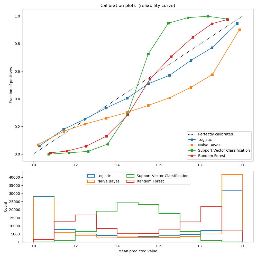
經過良好校準的分類器是概率分類器，它的輸出可以直接解釋為置信度。例如，經過良好校準的二分類器應該對樣本進行分類，這個樣本被給予的predict_proba值接近0.8，就意味著大約80%的把握屬于正類。

邏輯回歸返回良好的校準預測，因為它直接優化對數損失。相反，其他方法返回有偏概率，每種方法有不同的偏差：

GaussianNaiveBayes傾向于將概率推到0或1(注意直方圖中的計數)。這主要是因為它假設在給定類的情況下，特征是有條件獨立的，而在包含2個冗余特征的數據集中則不是這樣。
隨機森林分類器顯示相反的行為：直方圖顯示接近峰值。0.2和0.9的概率，而概率接近0或1是非常罕見的。Nculescu-Mizil和Caruana [1]給出了對此的解釋：“裝袋和隨機森林等方法--從一組基本模型的平均預測做出的預測接近0和1是很難的，因為底層基本模型中的方差會導致預測偏差，這些預測值本應該是0或者1，但是卻偏離了這些值。由于預測僅限于區間[0，1]，由方差引起的誤差往往是近0和1的單邊誤差。例如，如果一個模型應該對一個情況預測p=0，那么bagging法可以實現的唯一方法就是所有bagging中的樹都預測為零。如果將噪聲加到bagging中的樹木上，這種噪聲會導致一些樹預測值大于0，從而使bagging集合的平均預測值從0偏離。我們在隨機森林中觀察到的這種影響最強烈，因為使用隨機森林訓練的基層樹由于特征子集而具有較高的方差。“結果表明，校準曲線呈現出sigmoid形狀，表明分類器可以更多地信任它的“直覺”，并返回接近0或1的典型概率。
支持向量分類(SVC)顯示了一個比隨機森林分類器更加sigmoid形狀的曲線，這是典型的最大化間隔方法(比較Nculescu-Mizil和Caruana [1])，重點是關注那些接近決策邊界的硬樣本(支持向量)。

參考

1(1,2) Predicting Good Probabilities with Supervised Learning, A. Niculescu-Mizil & R. Caruana, ICML 2005

print(__doc__)

# Author: Jan Hendrik Metzen <jhm@informatik.uni-bremen.de>
# License: BSD Style.

import numpy as np
np.random.seed(0)

import matplotlib.pyplot as plt

from sklearn import datasets
from sklearn.naive_bayes import GaussianNB
from sklearn.linear_model import LogisticRegression
from sklearn.ensemble import RandomForestClassifier
from sklearn.svm import LinearSVC
from sklearn.calibration import calibration_curve

X, y = datasets.make_classification(n_samples=100000, n_features=20,
                                    n_informative=2, n_redundant=2)

train_samples = 100  # Samples used for training the models

X_train = X[:train_samples]
X_test = X[train_samples:]
y_train = y[:train_samples]
y_test = y[train_samples:]

# Create classifiers
lr = LogisticRegression()
gnb = GaussianNB()
svc = LinearSVC(C=1.0)
rfc = RandomForestClassifier()


# #############################################################################
# Plot calibration plots

plt.figure(figsize=(10, 10))
ax1 = plt.subplot2grid((3, 1), (0, 0), rowspan=2)
ax2 = plt.subplot2grid((3, 1), (2, 0))

ax1.plot([0, 1], [0, 1], "k:", label="Perfectly calibrated")
for clf, name in [(lr, 'Logistic'),
                  (gnb, 'Naive Bayes'),
                  (svc, 'Support Vector Classification'),
                  (rfc, 'Random Forest')]:
    clf.fit(X_train, y_train)
    if hasattr(clf, "predict_proba"):
        prob_pos = clf.predict_proba(X_test)[:, 1]
    else:  # use decision function
        prob_pos = clf.decision_function(X_test)
        prob_pos = \
            (prob_pos - prob_pos.min()) / (prob_pos.max() - prob_pos.min())
    fraction_of_positives, mean_predicted_value = \
        calibration_curve(y_test, prob_pos, n_bins=10)

    ax1.plot(mean_predicted_value, fraction_of_positives, "s-",
             label="%s" % (name, ))

    ax2.hist(prob_pos, range=(0, 1), bins=10, label=name,
             histtype="step", lw=2)

ax1.set_ylabel("Fraction of positives")
ax1.set_ylim([-0.05, 1.05])
ax1.legend(loc="lower right")
ax1.set_title('Calibration plots  (reliability curve)')

ax2.set_xlabel("Mean predicted value")
ax2.set_ylabel("Count")
ax2.legend(loc="upper center", ncol=2)

plt.tight_layout()
plt.show()

腳本的總運行時間：(0分1.370秒)