梯度提升回歸?

此示例演示了梯度提升從一組弱預測模型生成預測模型。梯度提升可以用于回歸和分類問題。在這里，我們將訓練一個模型來處理糖尿病回歸任務。我們將從梯度提升回歸器中得到結果， 這個梯度提升回歸器是使用最小二乘損失， 和500課深度為4的回歸樹組成。

注：對于較大的數據集(n_samples >= 10000)，請參閱sklearn.ensemble.HistGradientBoostingRegressor。

print(__doc__)

# Author: Peter Prettenhofer <peter.prettenhofer@gmail.com>
#         Maria Telenczuk <https://github.com/maikia>
#         Katrina Ni <https://github.com/nilichen>
#
# License: BSD 3 clause

import matplotlib.pyplot as plt
import numpy as np
from sklearn import datasets, ensemble
from sklearn.inspection import permutation_importance
from sklearn.metrics import mean_squared_error
from sklearn.model_selection import train_test_split

加載數據

首先，我們需要加載數據。

diabetes = datasets.load_diabetes()
X, y = diabetes.data, diabetes.target

數據預處理

接下來，我們將我們的數據集分割成90%用于訓練，剩下的用作測試。我們還將設置回歸模型的參數。您可以使用這些參數查看結果如何變化。

n_estimators :將執行的提升次數。稍后，我們將繪制反提升迭代的偏差。

max_depth :限制樹中的節點數。最佳的值取決于輸入變量之間的相互作用。

min_samples_split :內部節點分割時所需的最小樣本數。

learning_rate :每棵樹的貢獻會減少多少。

loss :損失函數優化。在這種情況下，使用最小二乘函數，但是還有許多其他選項。(看GradientBoostingRegressor)。

X_train, X_test, y_train, y_test = train_test_split(
    X, y, test_size=0.1, random_state=13)

params = {'n_estimators': 500,
          'max_depth': 4,
          'min_samples_split': 5,
          'learning_rate': 0.01,
          'loss': 'ls'}

擬合回歸模型

現在，我們將初始化一個梯度提升回歸器，并將其與我們的訓練數據進行擬合。讓我們也看看測試數據的均方誤差。

reg = ensemble.GradientBoostingRegressor(**params)
reg.fit(X_train, y_train)

mse = mean_squared_error(y_test, reg.predict(X_test))
print("The mean squared error (MSE) on test set: {:.4f}".format(mse))

The mean squared error (MSE) on test set: 3017.9419

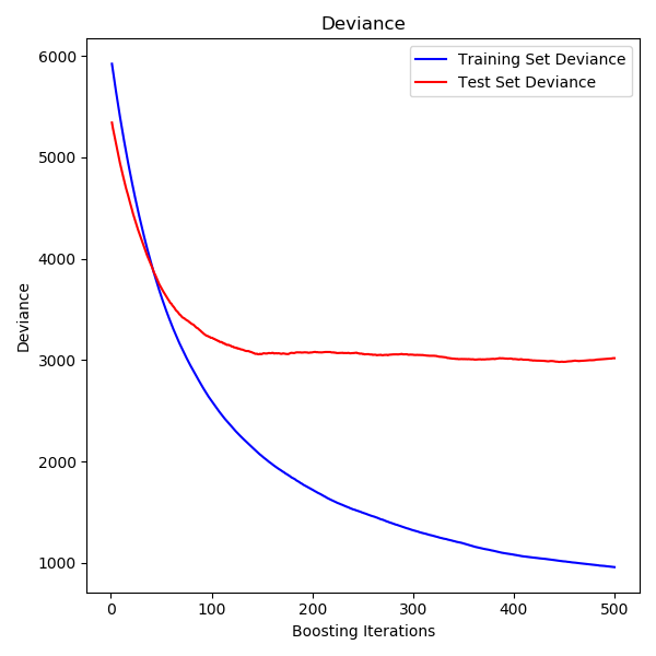
繪制訓練偏差

最后，我們將可視化結果。要做到這一點，我們將首先計算測試集偏差，然后根據提升迭代繪制測試集偏差圖。

test_score = np.zeros((params['n_estimators'],), dtype=np.float64)
for i, y_pred in enumerate(reg.staged_predict(X_test)):
    test_score[i] = reg.loss_(y_test, y_pred)

fig = plt.figure(figsize=(6, 6))
plt.subplot(1, 1, 1)
plt.title('Deviance')
plt.plot(np.arange(params['n_estimators']) + 1, reg.train_score_, 'b-',
         label='Training Set Deviance')
plt.plot(np.arange(params['n_estimators']) + 1, test_score, 'r-',
         label='Test Set Deviance')
plt.legend(loc='upper right')
plt.xlabel('Boosting Iterations')
plt.ylabel('Deviance')
fig.tight_layout()
plt.show()

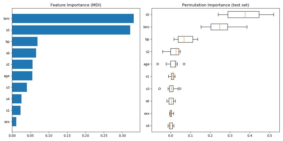
繪制特征重要性

小心一點、基于不純度的特征重要性對于高基數的特征(許多唯一的值)可能會產生誤導。作為一個替代項,reg的排列重要性可以在一個保持的測試集上計算。看Permutation feature importance更多細節。

在本例中，基于不純度和排列方法識別相同的2個強預測特征，但順序不同。第三大預測特征，“bp”，在這兩種方法中也是相同的。其余特征的預測性較低，排列圖中的錯誤條顯示它們與0重疊。

feature_importance = reg.feature_importances_
sorted_idx = np.argsort(feature_importance)
pos = np.arange(sorted_idx.shape[0]) + .5
fig = plt.figure(figsize=(12, 6))
plt.subplot(1, 2, 1)
plt.barh(pos, feature_importance[sorted_idx], align='center')
plt.yticks(pos, np.array(diabetes.feature_names)[sorted_idx])
plt.title('Feature Importance (MDI)')

result = permutation_importance(reg, X_test, y_test, n_repeats=10,
                                random_state=42, n_jobs=2)
sorted_idx = result.importances_mean.argsort()
plt.subplot(1, 2, 2)
plt.boxplot(result.importances[sorted_idx].T,
            vert=False, labels=np.array(diabetes.feature_names)[sorted_idx])
plt.title("Permutation Importance (test set)")
fig.tight_layout()
plt.show()

腳本的總運行時間：(0分2.168秒)

Download Python source code:plot_gradient_boosting_regression.py

Download Jupyter notebook:plot_gradient_boosting_regression.ipynb