普通最小二乘與嶺回歸差異?
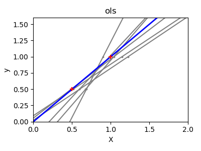
由于每個維度中的幾個點以及線性回歸所使用的直線盡可能地跟隨這些點,觀測數據上的噪聲將導致第一幅圖中所示的巨大差異。由于觀測中產生的噪聲,每條線的斜率對每個預測都會有很大的影響。
嶺回歸基本上是最小化最小二乘函數的懲罰版本。懲罰 shrinks了回歸系數的值。與標準線性回歸相比,盡管每個維的數據點較少,但預測的斜率要穩定得多,直線本身的方差也大大減小。

print(__doc__)


# Code source: Ga?l Varoquaux
# Modified for documentation by Jaques Grobler
# License: BSD 3 clause


import numpy as np
import matplotlib.pyplot as plt

from sklearn import linear_model

X_train = np.c_[.5, 1].T
y_train = [.5, 1]
X_test = np.c_[0, 2].T

np.random.seed(0)

classifiers = dict(ols=linear_model.LinearRegression(),
                   ridge=linear_model.Ridge(alpha=.1))

for name, clf in classifiers.items():
    fig, ax = plt.subplots(figsize=(4, 3))

    for _ in range(6):
        this_X = .1 * np.random.normal(size=(2, 1)) + X_train
        clf.fit(this_X, y_train)

        ax.plot(X_test, clf.predict(X_test), color='gray')
        ax.scatter(this_X, y_train, s=3, c='gray', marker='o', zorder=10)

    clf.fit(X_train, y_train)
    ax.plot(X_test, clf.predict(X_test), linewidth=2, color='blue')
    ax.scatter(X_train, y_train, s=30, c='red', marker='+', zorder=10)

    ax.set_title(name)
    ax.set_xlim(0, 2)
    ax.set_ylim((0, 1.6))
    ax.set_xlabel('X')
    ax.set_ylabel('y')

    fig.tight_layout()

plt.show()
腳本的總運行時間:(0分0.216秒)