使用Pipeline和GridSearchCV選擇降維算法?

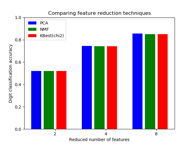
本示例構建了一個進行降維處理，然后使用支持向量分類器進行預測的管道。 它演示了如何使用GridSearchCV和Pipeline在單個CV運行中優化不同類別的估計量–在網格搜索過程中，將無監督的PCA和NMF降維與單變量特征進行了比較。

此外，可以使用memory參數實例化管道，以記住管道內的轉換器，從而避免反復安裝相同的轉換器。

請注意，當轉換器的安裝成本很高時，使用內存來啟用緩存就變得很有趣。

管道和GridSearchCV的展示

本節說明了將Pipeline與GridSearchCV一起使用。

# 作者: Robert McGibbon, Joel Nothman, Guillaume Lemaitre


import numpy as np
import matplotlib.pyplot as plt
from sklearn.datasets import load_digits
from sklearn.model_selection import GridSearchCV
from sklearn.pipeline import Pipeline
from sklearn.svm import LinearSVC
from sklearn.decomposition import PCA, NMF
from sklearn.feature_selection import SelectKBest, chi2

print(__doc__)

pipe = Pipeline([
    # the reduce_dim stage is populated by the param_grid
    ('reduce_dim', 'passthrough'),
    ('classify', LinearSVC(dual=False, max_iter=10000))
])

N_FEATURES_OPTIONS = [2, 4, 8]
C_OPTIONS = [1, 10, 100, 1000]
param_grid = [
    {
        'reduce_dim': [PCA(iterated_power=7), NMF()],
        'reduce_dim__n_components': N_FEATURES_OPTIONS,
        'classify__C': C_OPTIONS
    },
    {
        'reduce_dim': [SelectKBest(chi2)],
        'reduce_dim__k': N_FEATURES_OPTIONS,
        'classify__C': C_OPTIONS
    },
]
reducer_labels = ['PCA', 'NMF', 'KBest(chi2)']

grid = GridSearchCV(pipe, n_jobs=1, param_grid=param_grid)
X, y = load_digits(return_X_y=True)
grid.fit(X, y)

mean_scores = np.array(grid.cv_results_['mean_test_score'])
# 分數按param_grid迭代的順序排列，按字母順序排列
mean_scores = mean_scores.reshape(len(C_OPTIONS), -1, len(N_FEATURES_OPTIONS))
# 選擇最佳C的分數
mean_scores = mean_scores.max(axis=0)
bar_offsets = (np.arange(len(N_FEATURES_OPTIONS)) *
               (len(reducer_labels) + 1) + .5)

plt.figure()
COLORS = 'bgrcmyk'
for i, (label, reducer_scores) in enumerate(zip(reducer_labels, mean_scores)):
    plt.bar(bar_offsets + i, reducer_scores, label=label, color=COLORS[i])

plt.title("Comparing feature reduction techniques")
plt.xlabel('Reduced number of features')
plt.xticks(bar_offsets + len(reducer_labels) / 2, N_FEATURES_OPTIONS)
plt.ylabel('Digit classification accuracy')
plt.ylim((0, 1))
plt.legend(loc='upper left')

plt.show()

輸出：

在管道中緩存轉換器

有時值得存儲特定轉換器的狀態，因為它可以再次使用。 在GridSearchCV中使用管道會觸發這種情況。因此，我們使用參數內存（memory）來啟用緩存。

警告：請注意，此示例僅是示例，因為在這種特定情況下，擬合PCA不一定比加載緩存慢。 因此，當轉換器的安裝成本很高時，請使用內存構造函數參數。

from joblib import Memory
from shutil import rmtree

# 創建一個臨時文件夾來存儲管道的轉換器
location = 'cachedir'
memory = Memory(location=location, verbose=10)
cached_pipe = Pipeline([('reduce_dim', PCA()),
                        ('classify', LinearSVC(dual=False, max_iter=10000))],
                       memory=memory)

# 這次，將在網格搜索中使用緩存的管道

# 退出前刪除臨時緩存
memory.clear(warn=False)
rmtree(location)

僅在評估LinearSVC分類器的C參數的第一配置時計算PCA擬合。 ‘C’的其他配置將觸發緩存PCA估計器數據的加載，從而節省了處理時間。 因此，當安裝轉換器成本高昂時，使用內存對管道進行緩存非常有用。

腳本的總運行時間：（0分鐘5.976秒）