股市結構可視化?
此示例使用幾種無監督學習技術從歷史報價的變化中提取股票市場結構。
我們使用的數量是報價的每日變動:有關聯的報價往往在一天內波動。
學習一個圖結構
我們使用稀疏逆協方差估計來找出哪些報價是有條件相關的。具體來說,稀疏逆協方差給出了一個圖,它是一個連接列表。對于每個符號,它所連接的符號也是解釋其波動的有用符號。
聚類
我們使用聚類將行為類似的報價組合在一起。這里,在scikit-learn中可用的各種聚類技術中,我們使用了Affinity Propagation,因為它不強制執行大小相等的聚類,并且可以自動從數據中選擇聚類的數量。
請注意,這給出了與圖表不同的指示,因為圖表反映了變量之間的條件關系,而聚類則反映了邊際屬性:聚集在一起的變量在整個股票市場的水平上可以被認為具有類似的影響。
嵌入二維空間
為了便于可視化,我們需要在2D畫布上放置不同的符號。為此,我們使用Manifold learning技術檢索2D嵌入。
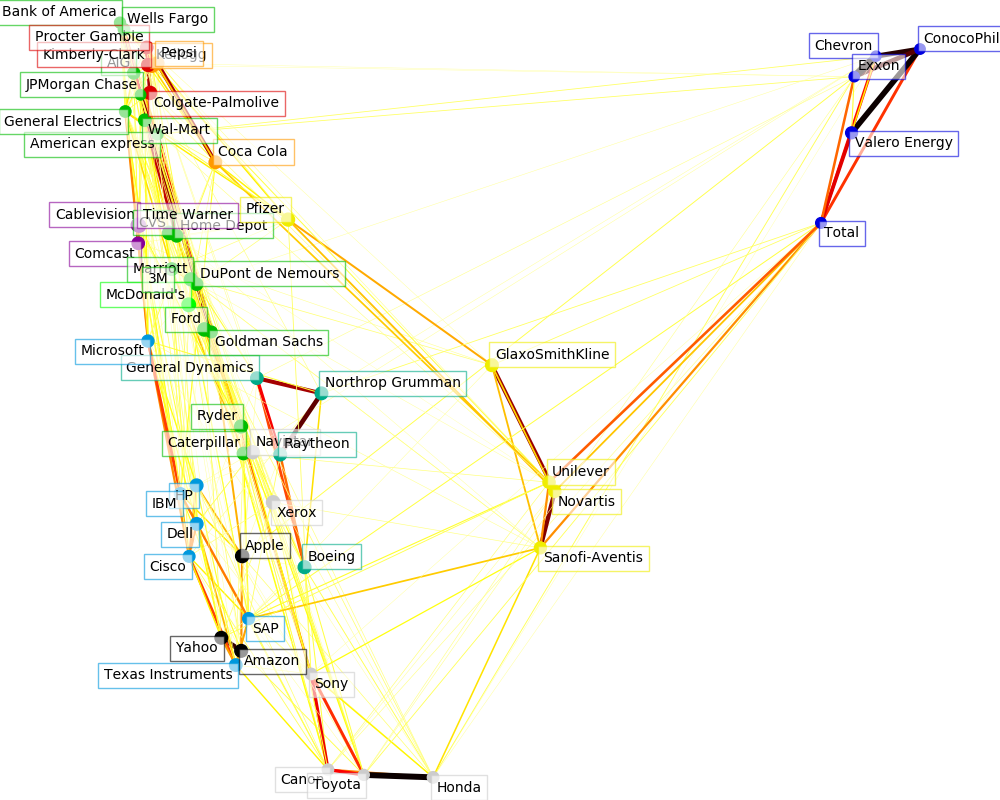
可視化
這三個模型的輸出組合在一個2D圖中,其中節點表示股票和邊界:
聚類標簽用于定義節點的顏色。 用稀疏協方差模型表示邊緣的強度。 2D嵌入用于在計劃中定位節點。
此示例包含大量與可視化相關的代碼,因為在這里可視化對于顯示圖形至關重要。其中一個挑戰是定位標簽盡量減少重疊。為此,我們使用了一種基于最近鄰沿每個軸的方向的啟發式方法。
Fetching quote history for 'AAPL'
Fetching quote history for 'AIG'
Fetching quote history for 'AMZN'
Fetching quote history for 'AXP'
Fetching quote history for 'BA'
Fetching quote history for 'BAC'
Fetching quote history for 'CAJ'
Fetching quote history for 'CAT'
Fetching quote history for 'CL'
Fetching quote history for 'CMCSA'
Fetching quote history for 'COP'
Fetching quote history for 'CSCO'
Fetching quote history for 'CVC'
Fetching quote history for 'CVS'
Fetching quote history for 'CVX'
Fetching quote history for 'DD'
Fetching quote history for 'DELL'
Fetching quote history for 'F'
Fetching quote history for 'GD'
Fetching quote history for 'GE'
Fetching quote history for 'GS'
Fetching quote history for 'GSK'
Fetching quote history for 'HD'
Fetching quote history for 'HMC'
Fetching quote history for 'HPQ'
Fetching quote history for 'IBM'
Fetching quote history for 'JPM'
Fetching quote history for 'K'
Fetching quote history for 'KMB'
Fetching quote history for 'KO'
Fetching quote history for 'MAR'
Fetching quote history for 'MCD'
Fetching quote history for 'MMM'
Fetching quote history for 'MSFT'
Fetching quote history for 'NAV'
Fetching quote history for 'NOC'
Fetching quote history for 'NVS'
Fetching quote history for 'PEP'
Fetching quote history for 'PFE'
Fetching quote history for 'PG'
Fetching quote history for 'R'
Fetching quote history for 'RTN'
Fetching quote history for 'SAP'
Fetching quote history for 'SNE'
Fetching quote history for 'SNY'
Fetching quote history for 'TM'
Fetching quote history for 'TOT'
Fetching quote history for 'TWX'
Fetching quote history for 'TXN'
Fetching quote history for 'UN'
Fetching quote history for 'VLO'
Fetching quote history for 'WFC'
Fetching quote history for 'WMT'
Fetching quote history for 'XOM'
Fetching quote history for 'XRX'
Fetching quote history for 'YHOO'
Cluster 1: Apple, Amazon, Yahoo
Cluster 2: Comcast, Cablevision, Time Warner
Cluster 3: ConocoPhillips, Chevron, Total, Valero Energy, Exxon
Cluster 4: Cisco, Dell, HP, IBM, Microsoft, SAP, Texas Instruments
Cluster 5: Boeing, General Dynamics, Northrop Grumman, Raytheon
Cluster 6: AIG, American express, Bank of America, Caterpillar, CVS, DuPont de Nemours, Ford, General Electrics, Goldman Sachs, Home Depot, JPMorgan Chase, Marriott, 3M, Ryder, Wells Fargo, Wal-Mart
Cluster 7: McDonald's
Cluster 8: GlaxoSmithKline, Novartis, Pfizer, Sanofi-Aventis, Unilever
Cluster 9: Kellogg, Coca Cola, Pepsi
Cluster 10: Colgate-Palmolive, Kimberly-Clark, Procter Gamble
Cluster 11: Canon, Honda, Navistar, Sony, Toyota, Xerox
# Author: Gael Varoquaux gael.varoquaux@normalesup.org
# License: BSD 3 clause

import sys

import numpy as np
import matplotlib.pyplot as plt
from matplotlib.collections import LineCollection

import pandas as pd

from sklearn import cluster, covariance, manifold

print(__doc__)


# #############################################################################
# Retrieve the data from Internet

# The data is from 2003 - 2008. This is reasonably calm: (not too long ago so
# that we get high-tech firms, and before the 2008 crash). This kind of
# historical data can be obtained for from APIs like the quandl.com and
# alphavantage.co ones.

symbol_dict = {
    'TOT': 'Total',
    'XOM': 'Exxon',
    'CVX': 'Chevron',
    'COP': 'ConocoPhillips',
    'VLO': 'Valero Energy',
    'MSFT': 'Microsoft',
    'IBM': 'IBM',
    'TWX': 'Time Warner',
    'CMCSA': 'Comcast',
    'CVC': 'Cablevision',
    'YHOO': 'Yahoo',
    'DELL': 'Dell',
    'HPQ': 'HP',
    'AMZN': 'Amazon',
    'TM': 'Toyota',
    'CAJ': 'Canon',
    'SNE': 'Sony',
    'F': 'Ford',
    'HMC': 'Honda',
    'NAV': 'Navistar',
    'NOC': 'Northrop Grumman',
    'BA': 'Boeing',
    'KO': 'Coca Cola',
    'MMM': '3M',
    'MCD': 'McDonald\'s',
    'PEP': 'Pepsi',
    'K': 'Kellogg',
    'UN': 'Unilever',
    'MAR': 'Marriott',
    'PG': 'Procter Gamble',
    'CL': 'Colgate-Palmolive',
    'GE': 'General Electrics',
    'WFC': 'Wells Fargo',
    'JPM': 'JPMorgan Chase',
    'AIG': 'AIG',
    'AXP': 'American express',
    'BAC': 'Bank of America',
    'GS': 'Goldman Sachs',
    'AAPL': 'Apple',
    'SAP': 'SAP',
    'CSCO': 'Cisco',
    'TXN': 'Texas Instruments',
    'XRX': 'Xerox',
    'WMT': 'Wal-Mart',
    'HD': 'Home Depot',
    'GSK': 'GlaxoSmithKline',
    'PFE': 'Pfizer',
    'SNY': 'Sanofi-Aventis',
    'NVS': 'Novartis',
    'KMB': 'Kimberly-Clark',
    'R': 'Ryder',
    'GD': 'General Dynamics',
    'RTN': 'Raytheon',
    'CVS': 'CVS',
    'CAT': 'Caterpillar',
    'DD': 'DuPont de Nemours'}


symbols, names = np.array(sorted(symbol_dict.items())).T

quotes = []

for symbol in symbols:
    print('Fetching quote history for %r' % symbol, file=sys.stderr)
    url = ('https://raw.githubusercontent.com/scikit-learn/examples-data/'
           'master/financial-data/{}.csv')
    quotes.append(pd.read_csv(url.format(symbol)))

close_prices = np.vstack([q['close'] for q in quotes])
open_prices = np.vstack([q['open'] for q in quotes])

# The daily variations of the quotes are what carry most information
variation = close_prices - open_prices


# #############################################################################
# Learn a graphical structure from the correlations
edge_model = covariance.GraphicalLassoCV()

# standardize the time series: using correlations rather than covariance
# is more efficient for structure recovery
X = variation.copy().T
X /= X.std(axis=0)
edge_model.fit(X)

# #############################################################################
# Cluster using affinity propagation

_, labels = cluster.affinity_propagation(edge_model.covariance_,
                                         random_state=0)
n_labels = labels.max()

for i in range(n_labels + 1):
    print('Cluster %i: %s' % ((i + 1), ', '.join(names[labels == i])))

# #############################################################################
# Find a low-dimension embedding for visualization: find the best position of
# the nodes (the stocks) on a 2D plane

# We use a dense eigen_solver to achieve reproducibility (arpack is
# initiated with random vectors that we don't control). In addition, we
# use a large number of neighbors to capture the large-scale structure.
node_position_model = manifold.LocallyLinearEmbedding(
    n_components=2, eigen_solver='dense', n_neighbors=6)

embedding = node_position_model.fit_transform(X.T).T

# #############################################################################
# Visualization
plt.figure(1, facecolor='w', figsize=(10, 8))
plt.clf()
ax = plt.axes([0., 0., 1., 1.])
plt.axis('off')

# Display a graph of the partial correlations
partial_correlations = edge_model.precision_.copy()
d = 1 / np.sqrt(np.diag(partial_correlations))
partial_correlations *= d
partial_correlations *= d[:, np.newaxis]
non_zero = (np.abs(np.triu(partial_correlations, k=1)) > 0.02)

# Plot the nodes using the coordinates of our embedding
plt.scatter(embedding[0], embedding[1], s=100 * d ** 2, c=labels,
            cmap=plt.cm.nipy_spectral)

# Plot the edges
start_idx, end_idx = np.where(non_zero)
# a sequence of (*line0*, *line1*, *line2*), where::
#            linen = (x0, y0), (x1, y1), ... (xm, ym)
segments = [[embedding[:, start], embedding[:, stop]]
            for start, stop in zip(start_idx, end_idx)]
values = np.abs(partial_correlations[non_zero])
lc = LineCollection(segments,
                    zorder=0, cmap=plt.cm.hot_r,
                    norm=plt.Normalize(0, .7 * values.max()))
lc.set_array(values)
lc.set_linewidths(15 * values)
ax.add_collection(lc)

# Add a label to each node. The challenge here is that we want to
# position the labels to avoid overlap with other labels
for index, (name, label, (x, y)) in enumerate(
        zip(names, labels, embedding.T)):

    dx = x - embedding[0]
    dx[index] = 1
    dy = y - embedding[1]
    dy[index] = 1
    this_dx = dx[np.argmin(np.abs(dy))]
    this_dy = dy[np.argmin(np.abs(dx))]
    if this_dx > 0:
        horizontalalignment = 'left'
        x = x + .002
    else:
        horizontalalignment = 'right'
        x = x - .002
    if this_dy > 0:
        verticalalignment = 'bottom'
        y = y + .002
    else:
        verticalalignment = 'top'
        y = y - .002
    plt.text(x, y, name, size=10,
             horizontalalignment=horizontalalignment,
             verticalalignment=verticalalignment,
             bbox=dict(facecolor='w',
                       edgecolor=plt.cm.nipy_spectral(label / float(n_labels)),
                       alpha=.6))

plt.xlim(embedding[0].min() - .15 * embedding[0].ptp(),
         embedding[0].max() + .10 * embedding[0].ptp(),)
plt.ylim(embedding[1].min() - .03 * embedding[1].ptp(),
         embedding[1].max() + .03 * embedding[1].ptp())

plt.show()
腳本的總運行時間:(0分9.212秒)