部分依賴圖?
部分依賴圖表示目標函數[2]與一組“目標”特征之間的依賴關系,在所有其他特征(補集特征)的值上邊際化。由于人類感知能力的限制,目標特征集的大小必須很小(通常是一兩個),因此目標特征通常是最重要的特征之一。
此示例演示如何從MLPRegressor和在加利福尼亞住房數據集上訓練的HistGradientBoostingRegressor獲取部分依賴圖。這個例子取自[1]。
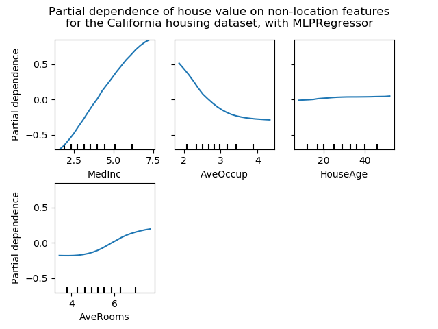
圖顯示四個 1-way 和兩個單向部分依賴圖(由于計算時間而被MLPRegressor省略)。單向PDP的目標變量是:中等收入(MedInc)、每戶平均住戶(AvgOccup)、中位住房年齡(HouseAge)和平均每戶房間(AveRooms)。
1 T. Hastie, R. Tibshirani and J. Friedman, “Elements of Statistical Learning Ed. 2”, Springer, 2009.
2 For classification you can think of it as the regression score before the link function.
print(__doc__)

from time import time
import numpy as np
import pandas as pd
import matplotlib.pyplot as plt
from mpl_toolkits.mplot3d import Axes3D

from sklearn.model_selection import train_test_split
from sklearn.preprocessing import QuantileTransformer
from sklearn.pipeline import make_pipeline

from sklearn.inspection import partial_dependence
from sklearn.inspection import plot_partial_dependence
from sklearn.experimental import enable_hist_gradient_boosting  # noqa
from sklearn.ensemble import HistGradientBoostingRegressor
from sklearn.neural_network import MLPRegressor
from sklearn.datasets import fetch_california_housing
California Housing數據集預處理
避免梯度提升偏差的中心目標:使用“遞歸”方法的梯度提升不考慮初始估計量(這里是平均目標,默認情況下)
cal_housing = fetch_california_housing()
X = pd.DataFrame(cal_housing.data, columns=cal_housing.feature_names)
y = cal_housing.target

y -= y.mean()

X_train, X_test, y_train, y_test = train_test_split(X, y, test_size=0.1,
                                                    random_state=0)
多層感知器的局部依賴計算
讓我們來擬合一個MLPRegressor,并計算單變量部分依賴圖。
print("Training MLPRegressor...")
tic = time()
est = make_pipeline(QuantileTransformer(),
                    MLPRegressor(hidden_layer_sizes=(50, 50),
                                 learning_rate_init=0.01,
                                 early_stopping=True))
est.fit(X_train, y_train)
print("done in {:.3f}s".format(time() - tic))
print("Test R2 score: {:.2f}".format(est.score(X_test, y_test)))
Training MLPRegressor...
done in 5.430s
Test R2 score: 0.81
我們配置了一條工作流來擴展數值輸入特征,并調整了神經網絡的大小和學習速率,從而在測試集上得到了訓練時間和預測性能之間的合理折衷。
重要的是,這個表格數據集因其特征而具有非常不同的動態范圍。神經網絡往往對不同尺度的特征非常敏感,而忽略了對數字特征的預處理,會導致一個非常糟糕的模型。
使用更大的神經網絡可以獲得更高的預測性能,但訓練成本也要高得多。
請注意,在繪制部分依賴之前,在測試集中檢查模型是否足夠準確是很重要的,因為在解釋給定特征對糟糕模型的預測功能的影響方面幾乎沒有用處。
現在讓我們使用模型不可知論(蠻力)方法計算這個神經網絡的部分依賴圖:
print('Computing partial dependence plots...')
tic = time()
# We don't compute the 2-way PDP (5, 1) here, because it is a lot slower
# with the brute method.
features = ['MedInc', 'AveOccup', 'HouseAge', 'AveRooms']
plot_partial_dependence(est, X_train, features,
                        n_jobs=3, grid_resolution=20)
print("done in {:.3f}s".format(time() - tic))
fig = plt.gcf()
fig.suptitle('Partial dependence of house value on non-location features\n'
             'for the California housing dataset, with MLPRegressor')
fig.subplots_adjust(hspace=0.3)
Computing partial dependence plots...
done in 3.392s
梯度提升的部分依賴計算
現在,我們來擬合一個GradientBoostingRegressor,計算部分依賴圖,或者一次計算一個或兩個變量。
print("Training GradientBoostingRegressor...")
tic = time()
est = HistGradientBoostingRegressor()
est.fit(X_train, y_train)
print("done in {:.3f}s".format(time() - tic))
print("Test R2 score: {:.2f}".format(est.score(X_test, y_test)))
Training GradientBoostingRegressor...
done in 0.757s
Test R2 score: 0.85
在這里,我們使用了梯度提升模型的默認超參數,而無需進行任何預處理,因為基于樹的模型對數值特征的單調變換具有很強的魯棒性。
請注意,在這個表格數據集上,梯度提升機的訓練速度和精度都比神經網絡快得多。調優它們的超參數也要便宜得多(默認參數往往運行良好,而神經網絡通常不是這樣)。
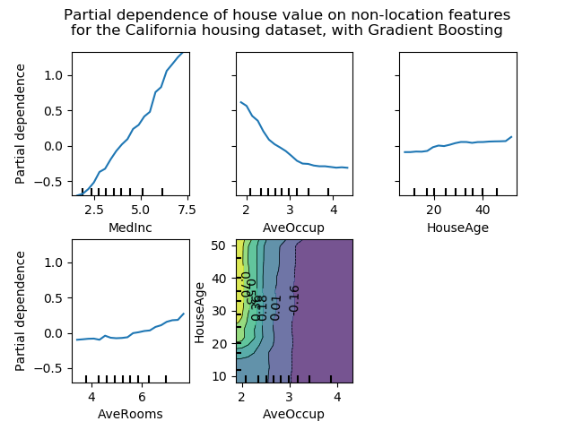
最后,正如我們接下來將看到的那樣,基于部分依賴圖樹的模型計算速度也快了幾個數量級,這使得為一對交互特征計算部分依賴圖的成本更低:
print('Computing partial dependence plots...')
tic = time()
features = ['MedInc', 'AveOccup', 'HouseAge', 'AveRooms',
            ('AveOccup', 'HouseAge')]
plot_partial_dependence(est, X_train, features,
                        n_jobs=3, grid_resolution=20)
print("done in {:.3f}s".format(time() - tic))
fig = plt.gcf()
fig.suptitle('Partial dependence of house value on non-location features\n'
             'for the California housing dataset, with Gradient Boosting')
fig.subplots_adjust(wspace=0.4, hspace=0.3)
Computing partial dependence plots...
done in 0.230s
圖分析
我們可以清楚地看到,中位房價與收入中位數(左上角)呈線性關系,當每個家庭的平均居住者增加(上、中)時,房價下降。右上角的顯示,一個地區的房屋年齡對房價(中位數)沒有很大的影響;每戶平均房數也是如此。x軸上的勾標表示訓練數據中特征值的十進制。
我們還觀察到 MLPRegressor比組HistGradientBoostingRegressor有更好的預測。為了使這些圖具有可比性,有必要減去目標y的平均值:默認情況下,用于組HistGradientBoostingRegressor的“遞歸”方法不考慮初始預測器(在本例中為平均目標)。將目標平均值設置為0可以避免這種偏差。
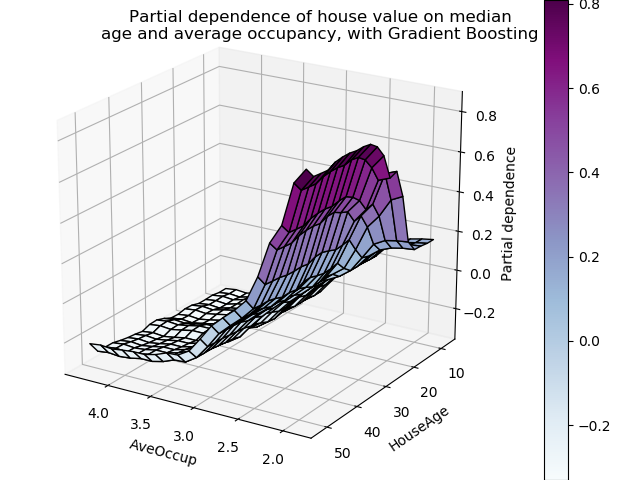
具有兩個目標特征的局部依賴圖使我們能夠可視化它們之間的交互作用。雙向部分依賴圖顯示了住宅價格中位數與住房年齡和平均居住者的共同值之間的相關性。我們可以清楚地看到這兩種特征之間的相互作用:對于平均入住率大于2的情況,房價幾乎與住房年齡無關,而對于小于2的價值,則對年齡有很強的依賴性。
三維交互圖
讓我們為這兩個特性的交互繪制同樣的部分依賴圖,這一次是在三維中。
fig = plt.figure()

features = ('AveOccup', 'HouseAge')
pdp, axes = partial_dependence(est, X_train, features=features,
                               grid_resolution=20)
XX, YY = np.meshgrid(axes[0], axes[1])
Z = pdp[0].T
ax = Axes3D(fig)
surf = ax.plot_surface(XX, YY, Z, rstride=1, cstride=1,
                       cmap=plt.cm.BuPu, edgecolor='k')
ax.set_xlabel(features[0])
ax.set_ylabel(features[1])
ax.set_zlabel('Partial dependence')
#  pretty init view
ax.view_init(elev=22, azim=122)
plt.colorbar(surf)
plt.suptitle('Partial dependence of house value on median\n'
             'age and average occupancy, with Gradient Boosting')
plt.subplots_adjust(top=0.9)

plt.show()
 腳本的總運行時間:(0分11.818秒)