線性模型系數解釋中的常見缺陷?

在線性模型中，目標值被建模為特征的線性組合(請參閱scikit-learn中“Linear Models 用戶指南”一節中對一組可用的線性模型的描述)。多個線性模型中的系數表示給定特征與目標之間的關系，假設所有其他特征保持不變(條件依賴)。這與繪制對和擬合線性關系不同：在這種情況下，其他特征的所有可能值都會在估計中得到考慮(邊際依賴)。

此示例將為解釋線性模型中的系數提供一些提示，指出當線性模型不適合描述數據集或當特征相關時會出現的問題。

我們會利用1985年的“目前人口統計調查”的數據，根據經驗、年齡或教育程度等各方面因素來預測工資。

• 數據集：工資
• 機器學習工作流
• 處理數據集
• 解釋系數：尺度問題
• 檢驗系數的可變性
• 關聯變量問題
• 預處理數值變量
• 正則化線性模型
• 稀疏系數的線性模型
• 課程學習

print(__doc__)

import numpy as np
import scipy as sp
import pandas as pd
import matplotlib.pyplot as plt
import seaborn as sns

數據集：工資

我們從OpenML獲取數據。注意，將參數 as_frame 設置為True， 將以pandas數據的形式檢索數據。

from sklearn.datasets import fetch_openml

survey = fetch_openml(data_id=534, as_frame=True)

然后，我們識別特征X和目標y：列WAGE是我們的目標變量(即我們想要預測的變量)。

X = survey.data[survey.feature_names]
X.describe(include="all")

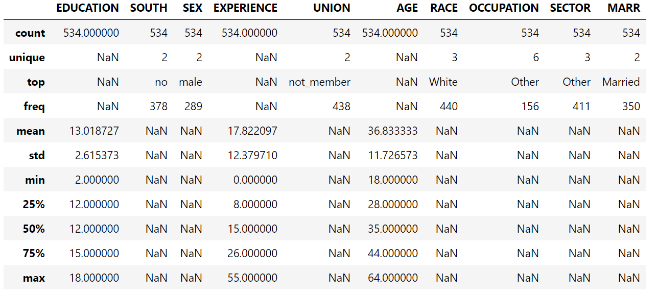注意，數據集包含分類變量和數值變量。在以后對數據集進行預處理時，我們需要考慮到這一點。

X.head()

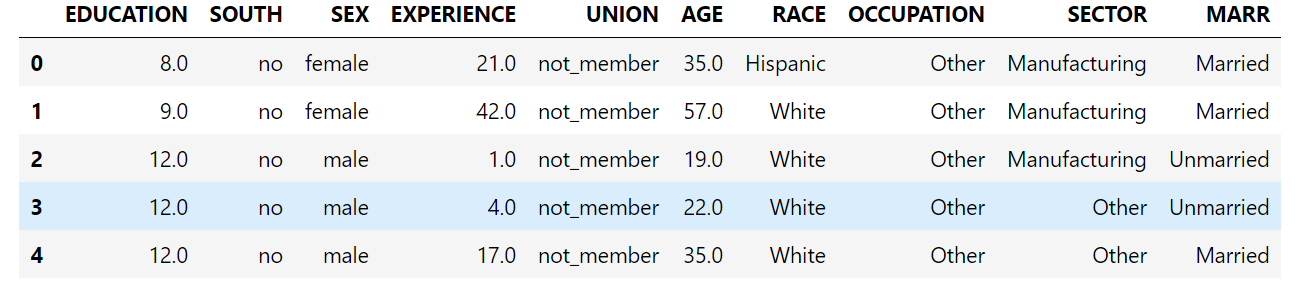我們的預測目標是：the wage。工資被描述為以每小時美元為單位的浮點數。

y = survey.target.values.ravel()
survey.target.head()

0    5.10
1    4.95
2    6.67
3    4.00
4    7.50
Name: WAGE, dtype: float64

我們將樣本分解成一個訓練集和一個測試集。只有訓練數據集將用于以下探索性分析。這是一種模擬在未知目標上執行預測的真實情況的方法，我們不希望我們的分析和決定因我們對測試數據有所了解而有偏差。

from sklearn.model_selection import train_test_split

X_train, X_test, y_train, y_test = train_test_split(
    X, y, random_state=42
)

首先，讓我們通過查看變量分布和它們之間的成對關系來獲得一些洞察力。只數值變量被使用。在下面的圖中，每個點表示一個示例。

train_dataset = X_train.copy()
train_dataset.insert(0, "WAGE", y_train)
_ = sns.pairplot(train_dataset, kind='reg', diag_kind='kde')

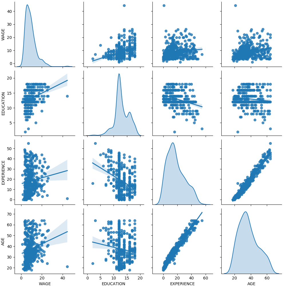仔細看一看工資分布，就會發現它是長尾的。因此，我們應該把它的對數近似地轉化為正態分布(線性模型，如嶺回歸或Lasso最適合用于正態分布的誤差)。

隨著 EDUCATION 的增加，WAGE 在增加。請注意，這里表示的工資和教育之間的依賴是邊際依賴，也就是說，它描述了一個特定變量的行為，而沒有保持其他變量的固定。

此外，EXPERIENCE 與 AGE 呈高度線性相關。

機器學習工作流

為了設計機器學習管道，我們首先手動檢查需要處理的數據類型：

survey.data.info()

<class 'pandas.core.frame.DataFrame'>
RangeIndex: 534 entries, 0 to 533
Data columns (total 10 columns):
 #   Column      Non-Null Count  Dtype
---  ------      --------------  -----
 0   EDUCATION   534 non-null    float64
 1   SOUTH       534 non-null    category
 2   SEX         534 non-null    category
 3   EXPERIENCE  534 non-null    float64
 4   UNION       534 non-null    category
 5   AGE         534 non-null    float64
 6   RACE        534 non-null    category
 7   OCCUPATION  534 non-null    category
 8   SECTOR      534 non-null    category
 9   MARR        534 non-null    category
dtypes: category(7), float64(3)
memory usage: 17.1 KB

如前所述，數據集包含具有不同數據類型的列，我們需要對每個數據類型應用特定的預處理。特別是，如果分類變量不首先編碼為整數，則不能將分類變量包括在線性模型中。此外，為了避免將分類特征視為有序值，我們需要對它們進行一次獨熱編碼。我們的預處理器：

• 獨熱編碼(即按類別生成一列)分類列；
• 作為第一種方法(我們將看到數值的標準化將如何影響我們的討論)，保持數值的原樣。

from sklearn.compose import make_column_transformer
from sklearn.preprocessing import OneHotEncoder

categorical_columns = ['RACE', 'OCCUPATION', 'SECTOR',
                       'MARR', 'UNION', 'SEX', 'SOUTH']
numerical_columns = ['EDUCATION', 'EXPERIENCE', 'AGE']

preprocessor = make_column_transformer(
    (OneHotEncoder(drop='if_binary'), categorical_columns),
    remainder='passthrough'
)

為了將數據集描述為線性模型，我們使用了一個正則化程度很小的嶺回歸，并對WAGE的對數進行了建模。

from sklearn.pipeline import make_pipeline
from sklearn.linear_model import Ridge
from sklearn.compose import TransformedTargetRegressor

model = make_pipeline(
    preprocessor,
    TransformedTargetRegressor(
        regressor=Ridge(alpha=1e-10),
        func=np.log10,
        inverse_func=sp.special.exp10
    )
)

處理數據集

首先，我們擬合模型。

_ = model.fit(X_train, y_train)

然后，我們檢查計算模型的性能，繪制它在測試集上的預測，并計算，例如，模型的中位絕對誤差。

from sklearn.metrics import median_absolute_error

y_pred = model.predict(X_train)

mae = median_absolute_error(y_train, y_pred)
string_score = f'MAE on training set: {mae:.2f} $/hour'
y_pred = model.predict(X_test)
mae = median_absolute_error(y_test, y_pred)
string_score += f'\nMAE on testing set: {mae:.2f} $/hour'
fig, ax = plt.subplots(figsize=(5, 5))
plt.scatter(y_test, y_pred)
ax.plot([0, 1], [0, 1], transform=ax.transAxes, ls="--", c="red")
plt.text(3, 20, string_score)
plt.title('Ridge model, small regularization')
plt.ylabel('Model predictions')
plt.xlabel('Truths')
plt.xlim([0, 27])
_ = plt.ylim([0, 27])

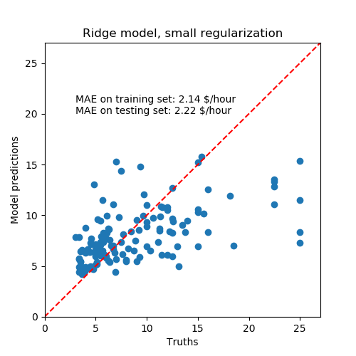學習到的模型遠不是一個做出準確預測的好模型：從上面的情節來看，這是顯而易見的，在那里，好的預測應該在紅線上。

在下一節中，我們將解釋模型的系數。當我們這樣做的時候，我們應該記住，我們得出的任何結論都是關于我們建立的模型，而不是關于數據的真實(現實世界)生成過程。

解釋系數：尺度問題

首先，我們可以查看我們所擬合的回歸系數的值。

feature_names = (model.named_steps['columntransformer']
                      .named_transformers_['onehotencoder']
                      .get_feature_names(input_features=categorical_columns))
feature_names = np.concatenate(
    [feature_names, numerical_columns])

coefs = pd.DataFrame(
    model.named_steps['transformedtargetregressor'].regressor_.coef_,
    columns=['Coefficients'], index=feature_names
)

coefs

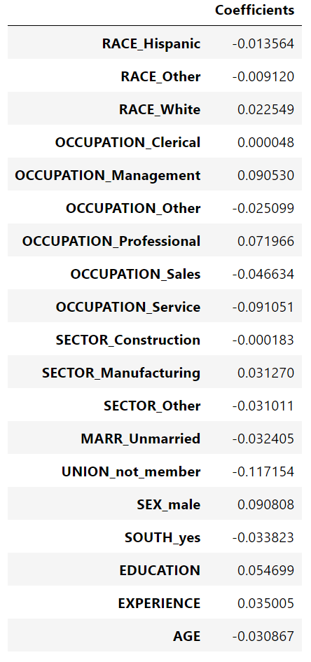年齡系數以“每活一年美元/小時”表示，而教育系數則以“每受教育一年美元/小時”表示。這個系數的表示說明了模型的實際預測：1歲的增長意味著每小時減少0.030867美元，而1年的教育增長意味著每小時增加0.054699美元。另一方面，范疇變量(如聯合變量或性別變量)是取值0或1的維數，其系數以美元/小時表示。然后，由于特征的度量單位不同，因此不能比較不同系數的大小，因為它們具有不同的自然尺度，因而具有不同的取值范圍。如果我們繪制系數，這是更明顯的。

coefs.plot(kind='barh', figsize=(9, 7))
plt.title('Ridge model, small regularization')
plt.axvline(x=0, color='.5')
plt.subplots_adjust(left=.3)

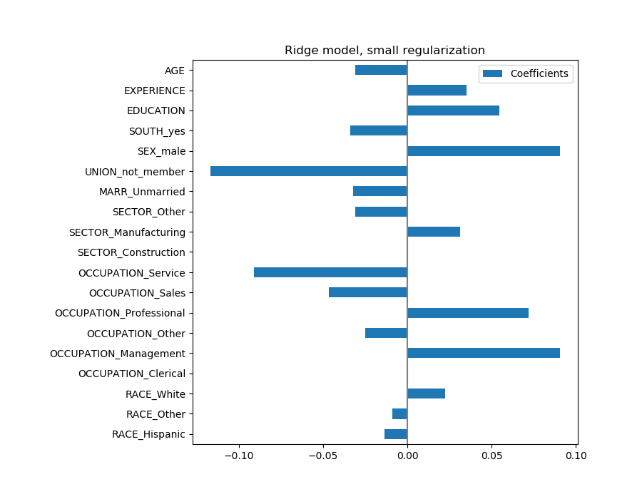事實上，從上面的圖來看，決定WAGE的最重要因素似乎是UNION，即使我們的直覺可能告訴我們，像 EXPERIENCE這樣的變量應該有更大的影響。

觀察系數圖來衡量特征的重要性可能會產生誤導，因為其中一些變化很小，而另一些，如AGE，變化更大，甚至幾十年。

如果我們比較不同特征的標準差，這是可見的。

X_train_preprocessed = pd.DataFrame(
    model.named_steps['columntransformer'].transform(X_train),
    columns=feature_names
)

X_train_preprocessed.std(axis=0).plot(kind='barh', figsize=(9, 7))
plt.title('Features std. dev.')
plt.subplots_adjust(left=.3)

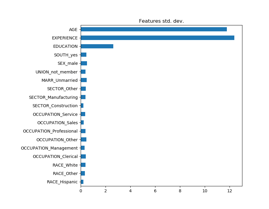將系數乘以相關特征的標準差，將所有系數減少到相同的度量單位。我們將看到，這相當于將數值變量標準化為其標準差，如:

在這種情況下，我們強調，特征的方差越大，輸出的相應系數的權重就越大，所有這些都是相等的。

coefs = pd.DataFrame(
    model.named_steps['transformedtargetregressor'].regressor_.coef_ *
    X_train_preprocessed.std(axis=0),
    columns=['Coefficient importance'], index=feature_names
)
coefs.plot(kind='barh', figsize=(9, 7))
plt.title('Ridge model, small regularization')
plt.axvline(x=0, color='.5')
plt.subplots_adjust(left=.3)

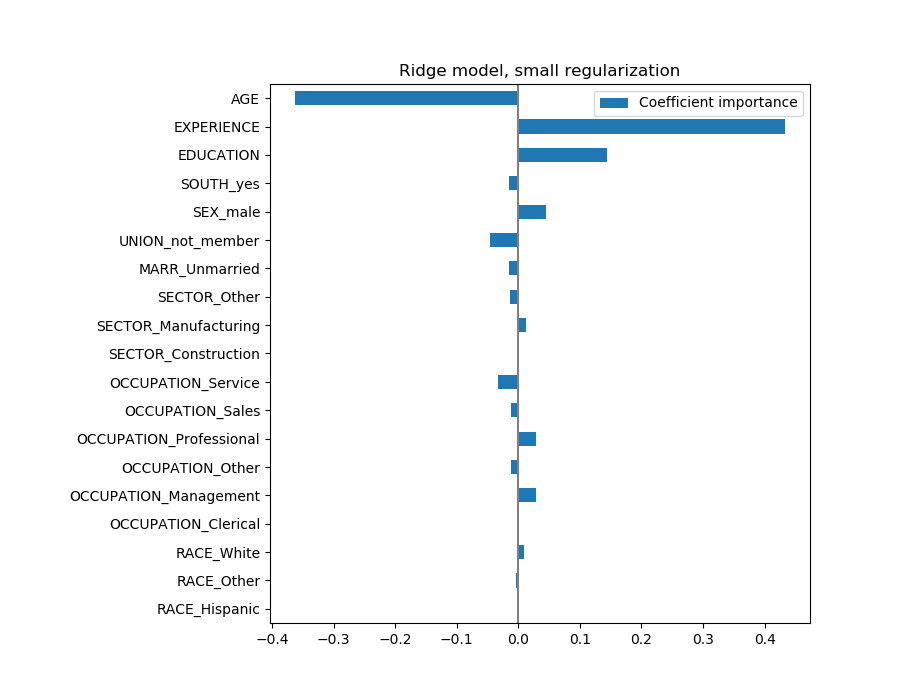現在系數已經被縮放了，我們可以安全地比較它們。

警告：為什么上面的情節意味著年齡的增長會導致工資的下降？為什么 initial pairplot告訴我們相反的情況？

上面的圖告訴我們，當所有其他特性保持不變(即條件依賴關系)時，特定特性與目標之間的依賴關系。即：條件依賴。當所有其他特征不變時，年齡的增加將導致工資的下降。相反，當所有其他特征不變時，經驗的增加會導致工資的增加。此外，年齡、經驗和教育是對模型影響最大的三個變量。

檢驗系數的可變性

我們可以通過交叉驗證來檢驗系數的可變性：它是數據擾動的一種形式(與重采樣有關)。

如果系數在改變輸入數據集時變化很大，則不能保證它們的魯棒性，因此很可能需要謹慎地解釋它們。

from sklearn.model_selection import cross_validate
from sklearn.model_selection import RepeatedKFold

cv_model = cross_validate(
    model, X, y, cv=RepeatedKFold(n_splits=5, n_repeats=5),
    return_estimator=True, n_jobs=-1
)
coefs = pd.DataFrame(
    [est.named_steps['transformedtargetregressor'].regressor_.coef_ *
     X_train_preprocessed.std(axis=0)
     for est in cv_model['estimator']],
    columns=feature_names
)
plt.figure(figsize=(9, 7))
sns.swarmplot(data=coefs, orient='h', color='k', alpha=0.5)
sns.boxplot(data=coefs, orient='h', color='cyan', saturation=0.5)
plt.axvline(x=0, color='.5')
plt.xlabel('Coefficient importance')
plt.title('Coefficient importance and its variability')
plt.subplots_adjust(left=.3)

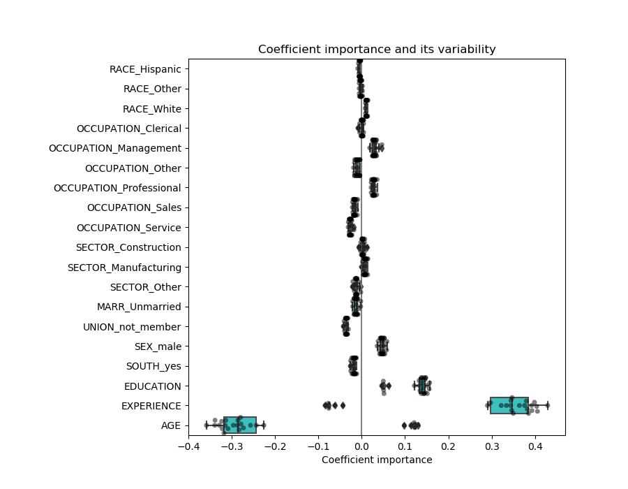
關聯變量問題

AGE和EXPERIENCE 系數受強變異性的影響，這可能是由于這兩個特征之間的共線性所致：由于AGE和EXPERIENCE在數據中的差異，它們的影響很難分開。

為了驗證這一解釋，我們繪制了年齡和經驗系數的變異性圖。

plt.ylabel('Age coefficient')
plt.xlabel('Experience coefficient')
plt.grid(True)
plt.xlim(-0.4, 0.5)
plt.ylim(-0.4, 0.5)
plt.scatter(coefs["AGE"], coefs["EXPERIENCE"])
_ = plt.title('Co-variations of coefficients for AGE and EXPERIENCE '
              'across folds')

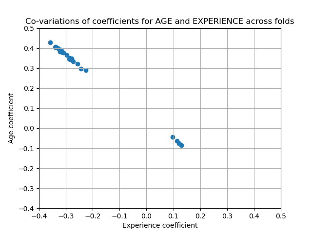有兩個區域：當EXPERIENCE系數為正值時，AGE為負，反之亦然。

為了更進一步，我們刪除了這兩個特征中的一個，并檢查了對模型穩定性的影響。

column_to_drop = ['AGE']

cv_model = cross_validate(
    model, X.drop(columns=column_to_drop), y,
    cv=RepeatedKFold(n_splits=5, n_repeats=5),
    return_estimator=True, n_jobs=-1
)
coefs = pd.DataFrame(
    [est.named_steps['transformedtargetregressor'].regressor_.coef_ *
     X_train_preprocessed.drop(columns=column_to_drop).std(axis=0)
     for est in cv_model['estimator']],
    columns=feature_names[:-1]
)
plt.figure(figsize=(9, 7))
sns.swarmplot(data=coefs, orient='h', color='k', alpha=0.5)
sns.boxplot(data=coefs, orient='h', color='cyan', saturation=0.5)
plt.axvline(x=0, color='.5')
plt.title('Coefficient importance and its variability')
plt.xlabel('Coefficient importance')
plt.subplots_adjust(left=.3)

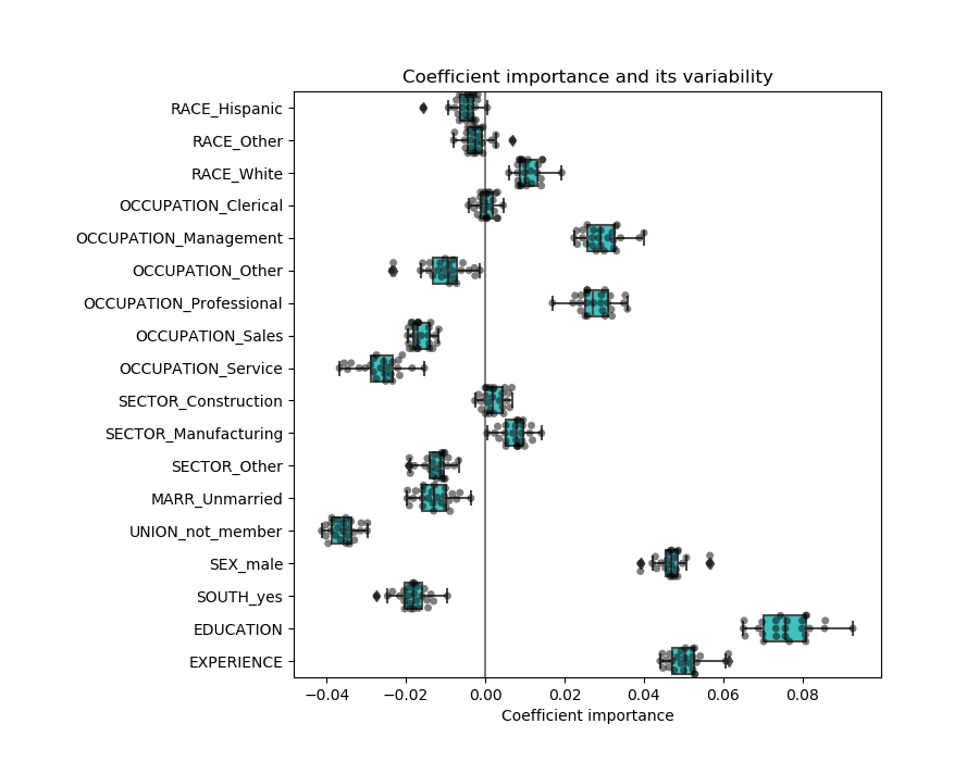經驗系數的估計現在變小了，對所有在交叉驗證過程中訓練的模型仍然很重要。

預處理數值變量

如前所述(請參閱“機器學習工作流”)，我們也可以選擇在訓練模型之前縮放數值。這將有助于將類似的數量正則化應用于嶺中的所有。為了將均值和尺度變化減去單位方差，對預處理器進行了重新定義。

from sklearn.preprocessing import StandardScaler

preprocessor = make_column_transformer(
    (OneHotEncoder(drop='if_binary'), categorical_columns),
    (StandardScaler(), numerical_columns),
    remainder='passthrough'
)

模型將保持不變。

model = make_pipeline(
    preprocessor,
    TransformedTargetRegressor(
        regressor=Ridge(alpha=1e-10),
        func=np.log10,
        inverse_func=sp.special.exp10
    )
)

_ = model.fit(X_train, y_train)

再次，我們用模型的中位絕對誤差和R方系數來檢驗計算模型的性能。

y_pred = model.predict(X_train)
mae = median_absolute_error(y_train, y_pred)
string_score = f'MAE on training set: {mae:.2f} $/hour'
y_pred = model.predict(X_test)
mae = median_absolute_error(y_test, y_pred)
string_score += f'\nMAE on testing set: {mae:.2f} $/hour'
fig, ax = plt.subplots(figsize=(6, 6))
plt.scatter(y_test, y_pred)
ax.plot([0, 1], [0, 1], transform=ax.transAxes, ls="--", c="red")

plt.text(3, 20, string_score)

plt.title('Ridge model, small regularization, normalized variables')
plt.ylabel('Model predictions')
plt.xlabel('Truths')
plt.xlim([0, 27])
_ = plt.ylim([0, 27])

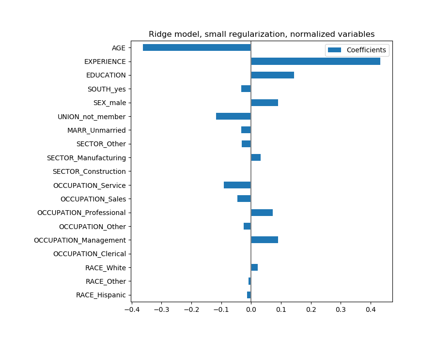
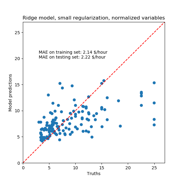對于系數分析，這次不需要縮放。

coefs = pd.DataFrame(
    model.named_steps['transformedtargetregressor'].regressor_.coef_,
    columns=['Coefficients'], index=feature_names
)
coefs.plot(kind='barh', figsize=(9, 7))
plt.title('Ridge model, small regularization, normalized variables')
plt.axvline(x=0, color='.5')
plt.subplots_adjust(left=.3)

我們現在檢查幾個交叉驗證的系數。

cv_model = cross_validate(
    model, X, y, cv=RepeatedKFold(n_splits=5, n_repeats=5),
    return_estimator=True, n_jobs=-1
)
coefs = pd.DataFrame(
    [est.named_steps['transformedtargetregressor'].regressor_.coef_
     for est in cv_model['estimator']],
    columns=feature_names
)
plt.figure(figsize=(9, 7))
sns.swarmplot(data=coefs, orient='h', color='k', alpha=0.5)
sns.boxplot(data=coefs, orient='h', color='cyan', saturation=0.5)
plt.axvline(x=0, color='.5')
plt.title('Coefficient variability')
plt.subplots_adjust(left=.3)

結果與非歸一化情況十分相似。

正則化線性模型

在機器學習實踐中，嶺回歸更常用于不可忽略的正則化。

上面，我們把這個正規化限制在很小的數量上。正則化改善了問題的條件，減少了估計的方差。RidgeCV應用交叉驗證來確定正則化參數(Alpha)的哪個值最適合于預測。

from sklearn.linear_model import RidgeCV

model = make_pipeline(
    preprocessor,
    TransformedTargetRegressor(
        regressor=RidgeCV(alphas=np.logspace(-10, 10, 21)),
        func=np.log10,
        inverse_func=sp.special.exp10
    )
)

_ = model.fit(X_train, y_train)

首先，我們檢查選擇了哪個值的α。

model[-1].regressor_.alpha_

然后我們檢查預測的質量。

y_pred = model.predict(X_train)
mae = median_absolute_error(y_train, y_pred)
string_score = f'MAE on training set: {mae:.2f} $/hour'
y_pred = model.predict(X_test)
mae = median_absolute_error(y_test, y_pred)
string_score += f'\nMAE on testing set: {mae:.2f} $/hour'

fig, ax = plt.subplots(figsize=(6, 6))
plt.scatter(y_test, y_pred)
ax.plot([0, 1], [0, 1], transform=ax.transAxes, ls="--", c="red")

plt.text(3, 20, string_score)

plt.title('Ridge model, regularization, normalized variables')
plt.ylabel('Model predictions')
plt.xlabel('Truths')
plt.xlim([0, 27])
_ = plt.ylim([0, 27])

正則化模型的數據再現能力與非正則模型相似。

coefs = pd.DataFrame(
    model.named_steps['transformedtargetregressor'].regressor_.coef_,
    columns=['Coefficients'], index=feature_names
)
coefs.plot(kind='barh', figsize=(9, 7))
plt.title('Ridge model, regularization, normalized variables')
plt.axvline(x=0, color='.5')
plt.subplots_adjust(left=.3)

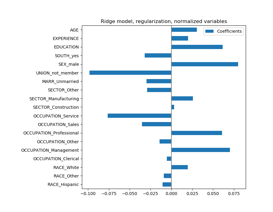這些系數有顯著性差異。年齡和經驗系數都是正的，但它們現在對預測的影響較小。

正則化減少了相關變量對模型的影響，因為權重在兩個預測變量之間是共享的，因此兩者都不會有很強的權重。

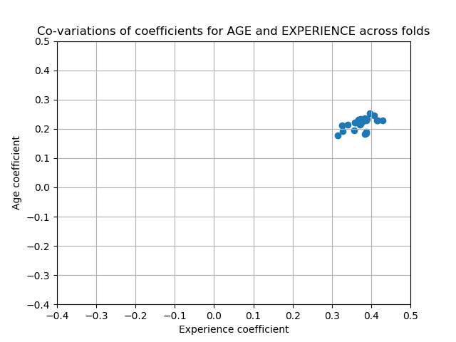
另一方面，正則化獲得的權重更穩定(參見嶺回歸和分類用戶指南一節)。在交叉驗證中，從從數據擾動中獲得的圖中可以看出這種增加的穩定性。這個圖可以和前一個相比較。

cv_model = cross_validate(
    model, X, y, cv=RepeatedKFold(n_splits=5, n_repeats=5),
    return_estimator=True, n_jobs=-1
)
coefs = pd.DataFrame(
    [est.named_steps['transformedtargetregressor'].regressor_.coef_ *
     X_train_preprocessed.std(axis=0)
     for est in cv_model['estimator']],
    columns=feature_names
)

plt.ylabel('Age coefficient')
plt.xlabel('Experience coefficient')
plt.grid(True)
plt.xlim(-0.4, 0.5)
plt.ylim(-0.4, 0.5)
plt.scatter(coefs["AGE"], coefs["EXPERIENCE"])
_ = plt.title('Co-variations of coefficients for AGE and EXPERIENCE '
              'across folds')

稀疏系數的線性模型

在數據集中考慮相關變量的另一種可能性是估計稀疏系數。在某種程度上，當我們在以前的嶺估計中刪除AGE列時，我們已經手動完成了。

LASSO模型(見Lasso用戶指南部分)估計稀疏系數。LassoCV應用交叉驗證來確定正則化參數(Alpha)的哪個值最適合于模型估計。

from sklearn.linear_model import LassoCV

model = make_pipeline(
    preprocessor,
    TransformedTargetRegressor(
        regressor=LassoCV(alphas=np.logspace(-10, 10, 21), max_iter=100000),
        func=np.log10,
        inverse_func=sp.special.exp10
    )
)

_ = model.fit(X_train, y_train)

首先，我們檢查了選擇了哪個值的α。

model[-1].regressor_.alpha_

0.001

然后我們檢查預測的質量。

y_pred = model.predict(X_train)
mae = median_absolute_error(y_train, y_pred)
string_score = f'MAE on training set: {mae:.2f} $/hour'
y_pred = model.predict(X_test)
mae = median_absolute_error(y_test, y_pred)
string_score += f'\nMAE on testing set: {mae:.2f} $/hour'

fig, ax = plt.subplots(figsize=(6, 6))
plt.scatter(y_test, y_pred)
ax.plot([0, 1], [0, 1], transform=ax.transAxes, ls="--", c="red")

plt.text(3, 20, string_score)

plt.title('Lasso model, regularization, normalized variables')
plt.ylabel('Model predictions')
plt.xlabel('Truths')
plt.xlim([0, 27])
_ = plt.ylim([0, 27])

同樣，對于我們的數據集，模型也不是很有預見性。

coefs = pd.DataFrame(
    model.named_steps['transformedtargetregressor'].regressor_.coef_,
    columns=['Coefficients'], index=feature_names
)
coefs.plot(kind='barh', figsize=(9, 7))
plt.title('Lasso model, regularization, normalized variables')
plt.axvline(x=0, color='.5')
plt.subplots_adjust(left=.3)

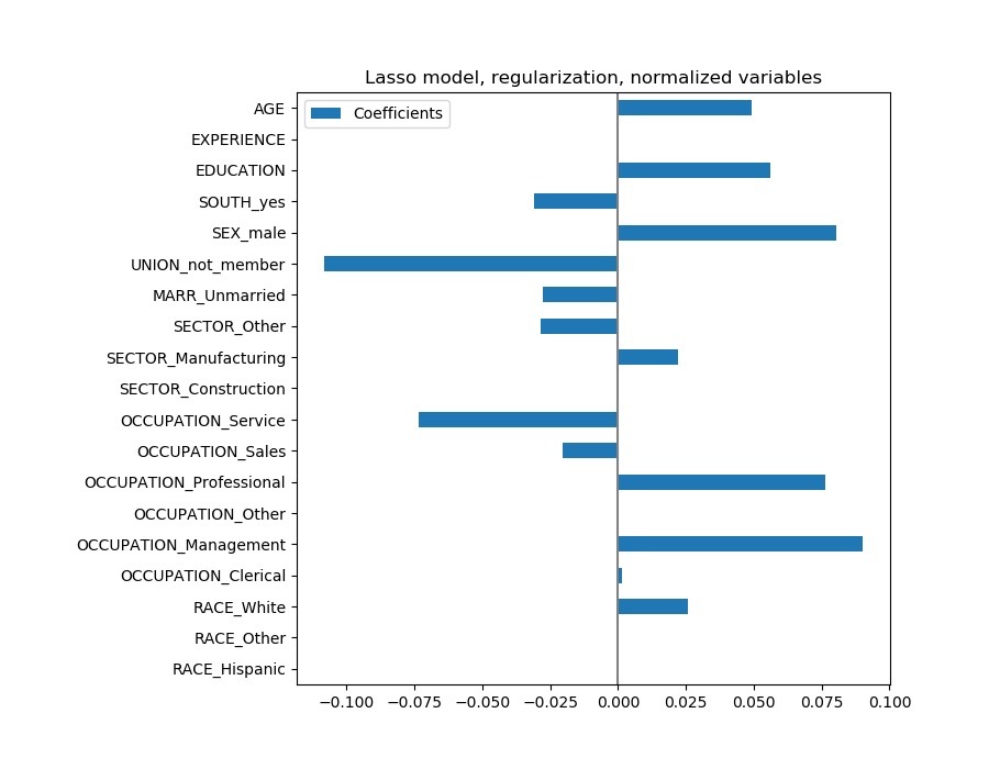Lasso模型識別了年齡和經驗之間的相關性，并為了預測而壓制其中一個。

重要的是要記住，被丟棄的系數可能仍然與結果本身有關：模型選擇了抑制它們，因為它們在其他特征之上很少或沒有額外的信息。

課程學習

• 要檢索特征重要性，系數必須縮放到相同的度量單位。使用特性的標準差對它們進行縮放是一個有用的代理。
• 多元線性模型中的系數表示給定特征與目標之間的依賴關系，這有賴于其他特征。
• 相關特征導致線性模型系數不穩定，其影響不能很好地分解。
• 不同的線性模型對特征相關性的響應不同，各相關系數可能存在顯著差異。
• 通過交叉驗證循環對系數進行檢測，給出了它們的穩定性概念。

腳本的總運行時間：(0分21.601秒)。

Download Python source code: plot_linear_model_coefficient_interpretation.py

Download Jupyter notebook: plot_linear_model_coefficient_interpretation.ipynb