核嶺回歸與SVR的比較?

內核嶺回歸（KRR）和SVR都通過采用內核技巧來學習非線性函數，即，它們在由相應內核誘導的空間中學習了與原始空間中的非線性函數相對應的線性函數。它們在損失函數上有所不同（脊波與對ε無關的損失）。與SVR相比，KRR的擬合可以封閉形式進行，對于中等規模的數據集通常更快。另一方面，學習的模型是非稀疏的，因此在預測時比SVR慢。

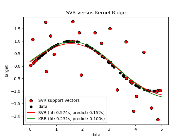
此示例說明了人工數據集上的兩種方法，該方法由正弦目標函數和添加到每五個數據點的強噪聲組成。第一張圖比較了當使用網格搜索優化RBF內核的復雜度/正則化和帶寬時，KRR和SVR的學習模型。學習的功能非常相似。但是，擬合KRR約為。比安裝SVR快7倍（兩者都使用網格搜索）。但是，使用SVR預測100000個目標值的速度快了樹倍以上，因為它僅使用了大約10個像素就學會了稀疏模型。 100個訓練數據點的1/3作為支持向量。

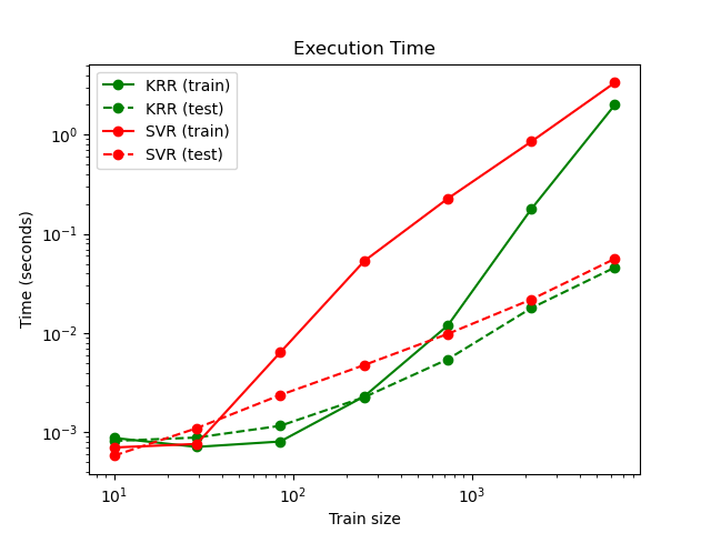
下圖比較了不同大小的訓練集的KRR和SVR的擬合和預測時間。對于中型訓練集（少于1000個樣本），擬合KRR比SVR快。但是，對于較大的訓練集，SVR的縮放范圍更好。關于預測時間，由于學習到的稀疏解決方案，對于所有規模的訓練集，SVR均比KRR更快。注意，稀疏度以及預測時間取決于SVR的參數ε和C。

# 作者: Jan Hendrik Metzen <jhm@informatik.uni-bremen.de>
# 執照: BSD 3 clause


import time

import numpy as np

from sklearn.svm import SVR
from sklearn.model_selection import GridSearchCV
from sklearn.model_selection import learning_curve
from sklearn.kernel_ridge import KernelRidge
import matplotlib.pyplot as plt

rng = np.random.RandomState(0)

# #############################################################################
# 獲得樣本數據
X = 5 * rng.rand(10000, 1)
y = np.sin(X).ravel()

# 對目標增加噪音
y[::5] += 3 * (0.5 - rng.rand(X.shape[0] // 5))

X_plot = np.linspace(0, 5, 100000)[:, None]

# #############################################################################
# 擬合回歸模型
train_size = 100
svr = GridSearchCV(SVR(kernel='rbf', gamma=0.1),
                   param_grid={"C": [1e0, 1e1, 1e2, 1e3],
                               "gamma": np.logspace(-2, 2, 5)})

kr = GridSearchCV(KernelRidge(kernel='rbf', gamma=0.1),
                  param_grid={"alpha": [1e0, 0.1, 1e-2, 1e-3],
                              "gamma": np.logspace(-2, 2, 5)})

t0 = time.time()
svr.fit(X[:train_size], y[:train_size])
svr_fit = time.time() - t0
print("SVR complexity and bandwidth selected and model fitted in %.3f s"
      % svr_fit)

t0 = time.time()
kr.fit(X[:train_size], y[:train_size])
kr_fit = time.time() - t0
print("KRR complexity and bandwidth selected and model fitted in %.3f s"
      % kr_fit)

sv_ratio = svr.best_estimator_.support_.shape[0] / train_size
print("Support vector ratio: %.3f" % sv_ratio)

t0 = time.time()
y_svr = svr.predict(X_plot)
svr_predict = time.time() - t0
print("SVR prediction for %d inputs in %.3f s"
      % (X_plot.shape[0], svr_predict))

t0 = time.time()
y_kr = kr.predict(X_plot)
kr_predict = time.time() - t0
print("KRR prediction for %d inputs in %.3f s"
      % (X_plot.shape[0], kr_predict))


# #############################################################################
# 查看結果
sv_ind = svr.best_estimator_.support_
plt.scatter(X[sv_ind], y[sv_ind], c='r', s=50, label='SVR support vectors',
            zorder=2, edgecolors=(0, 0, 0))
plt.scatter(X[:100], y[:100], c='k', label='data', zorder=1,
            edgecolors=(0, 0, 0))
plt.plot(X_plot, y_svr, c='r',
         label='SVR (fit: %.3fs, predict: %.3fs)' % (svr_fit, svr_predict))
plt.plot(X_plot, y_kr, c='g',
         label='KRR (fit: %.3fs, predict: %.3fs)' % (kr_fit, kr_predict))
plt.xlabel('data')
plt.ylabel('target')
plt.title('SVR versus Kernel Ridge')
plt.legend()

# 可視化訓練和預測時間
plt.figure()

# 獲取樣本數據
X = 5 * rng.rand(10000, 1)
y = np.sin(X).ravel()
y[::5] += 3 * (0.5 - rng.rand(X.shape[0] // 5))
sizes = np.logspace(1, 4, 7).astype(np.int)
for name, estimator in {"KRR": KernelRidge(kernel='rbf', alpha=0.1,
                                           gamma=10),
                        "SVR": SVR(kernel='rbf', C=1e1, gamma=10)}.items():
    train_time = []
    test_time = []
    for train_test_size in sizes:
        t0 = time.time()
        estimator.fit(X[:train_test_size], y[:train_test_size])
        train_time.append(time.time() - t0)

        t0 = time.time()
        estimator.predict(X_plot[:1000])
        test_time.append(time.time() - t0)

    plt.plot(sizes, train_time, 'o-', color="r" if name == "SVR" else "g",
             label="%s (train)" % name)
    plt.plot(sizes, test_time, 'o--', color="r" if name == "SVR" else "g",
             label="%s (test)" % name)

plt.xscale("log")
plt.yscale("log")
plt.xlabel("Train size")
plt.ylabel("Time (seconds)")
plt.title('Execution Time')
plt.legend(loc="best")

# 可視化學習曲線
plt.figure()

svr = SVR(kernel='rbf', C=1e1, gamma=0.1)
kr = KernelRidge(kernel='rbf', alpha=0.1, gamma=0.1)
train_sizes, train_scores_svr, test_scores_svr = \
    learning_curve(svr, X[:100], y[:100], train_sizes=np.linspace(0.1, 1, 10),
                   scoring="neg_mean_squared_error", cv=10)
train_sizes_abs, train_scores_kr, test_scores_kr = \
    learning_curve(kr, X[:100], y[:100], train_sizes=np.linspace(0.1, 1, 10),
                   scoring="neg_mean_squared_error", cv=10)

plt.plot(train_sizes, -test_scores_svr.mean(1), 'o-', color="r",
         label="SVR")
plt.plot(train_sizes, -test_scores_kr.mean(1), 'o-', color="g",
         label="KRR")
plt.xlabel("Train size")
plt.ylabel("Mean Squared Error")
plt.title('Learning curves')
plt.legend(loc="best")

plt.show()

輸出：

SVR complexity and bandwidth selected and model fitted in 0.751 s
KRR complexity and bandwidth selected and model fitted in 0.241 s
Support vector ratio: 0.320
SVR prediction for 100000 inputs in 0.120 s
KRR prediction for 100000 inputs in 0.381 s

腳本的總運行時間：（0分鐘23.567秒）