使用IterativeImputer的變體估算缺失值?
sklearn.impute.IterativeImputer類非常靈活:它可以與各種估算器一起使用以進行循環回歸,將每個變量依次作為輸出。
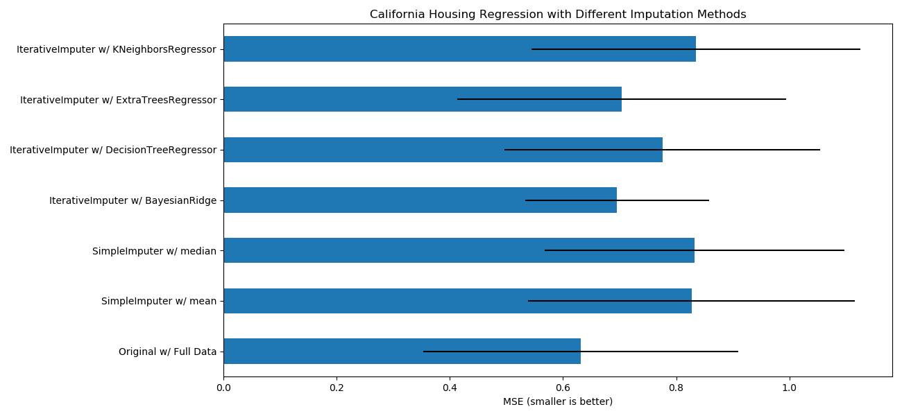
在此示例中,我們將一些估計器與sklearn.impute.IterativeImputer進行了比較,以估計缺失的特征:
BayesianRidge:貝葉斯領回歸,一種正則線性回歸
DecisionTreeRegressor:決策樹回歸,非線性回歸
ExtraTreesRegressor:額外樹回歸,類似于R中的missForest
KNeighborsRegressor:K近鄰回歸,與其他KNN插補方法相當
特別令人感興趣的是sklearn.impute.IterativeImputer用以模仿missForest(R的流行插補包)行為的功能。在此示例中,我們選擇使用sklearn.ensemble.ExtraTreesRegressor而不是sklearn.ensemble.RandomForestRegressor(如missForest),因為它提高了速度。
請注意,sklearn.neighbors.KNeighborsRegressor與KNN插補不同,后者通過使用考慮缺失值而不是插補的距離度量從缺失值的樣本中學習。
目標是比較不同的估算器,以查看在加利福尼亞住房數據集中使用sklearn.linear_model.BayesianRidge估算器時,哪一個最適合sklearn.impute.IterativeImputer,并且從各行中隨機刪除一個值。
對于這種特殊的缺失值模式,我們看到sklearn.ensemble.ExtraTreesRegressor和sklearn.linear_model.BayesianRidge提供了最佳結果。
輸入:
print(__doc__)

import numpy as np
import matplotlib.pyplot as plt
import pandas as pd

# 要使用此實驗特性,我們需要明確引入以下包和庫:
from sklearn.experimental import enable_iterative_imputer  # noqa
from sklearn.datasets import fetch_california_housing
from sklearn.impute import SimpleImputer
from sklearn.impute import IterativeImputer
from sklearn.linear_model import BayesianRidge
from sklearn.tree import DecisionTreeRegressor
from sklearn.ensemble import ExtraTreesRegressor
from sklearn.neighbors import KNeighborsRegressor
from sklearn.pipeline import make_pipeline
from sklearn.model_selection import cross_val_score

N_SPLITS = 5

rng = np.random.RandomState(0)

X_full, y_full = fetch_california_housing(return_X_y=True)
# 就示例而言,大約2k個樣本就足夠了。
# 刪除以下兩行,能夠使運行速度因不同的錯誤條而放慢。
X_full = X_full[::10]
y_full = y_full[::10]
n_samples, n_features = X_full.shape

# 估計整個數據集的分數,沒有缺失值
br_estimator = BayesianRidge()
score_full_data = pd.DataFrame(
    cross_val_score(
        br_estimator, X_full, y_full, scoring='neg_mean_squared_error',
        cv=N_SPLITS
    ),
    columns=['Full Data']
)

# 每行添加一個缺失值
X_missing = X_full.copy()
y_missing = y_full
missing_samples = np.arange(n_samples)
missing_features = rng.choice(n_features, n_samples, replace=True)
X_missing[missing_samples, missing_features] = np.nan

# 估算插補后的得分(均值和中位數策略)
score_simple_imputer = pd.DataFrame()
for strategy in ('mean', 'median'):
    estimator = make_pipeline(
        SimpleImputer(missing_values=np.nan, strategy=strategy),
        br_estimator
    )
    score_simple_imputer[strategy] = cross_val_score(
        estimator, X_missing, y_missing, scoring='neg_mean_squared_error',
        cv=N_SPLITS
    )

# 在用不同的估計量迭代插補缺失值之后估計分數
estimators = [
    BayesianRidge(),
    DecisionTreeRegressor(max_features='sqrt', random_state=0),
    ExtraTreesRegressor(n_estimators=10, random_state=0),
    KNeighborsRegressor(n_neighbors=15)
]
score_iterative_imputer = pd.DataFrame()
for impute_estimator in estimators:
    estimator = make_pipeline(
        IterativeImputer(random_state=0, estimator=impute_estimator),
        br_estimator
    )
    score_iterative_imputer[impute_estimator.__class__.__name__] = \
        cross_val_score(
            estimator, X_missing, y_missing, scoring='neg_mean_squared_error',
            cv=N_SPLITS
        )

scores = pd.concat(
    [score_full_data, score_simple_imputer, score_iterative_imputer],
    keys=['Original', 'SimpleImputer', 'IterativeImputer'], axis=1
)

# 繪制加利福尼亞房屋價值數據集上的結果
fig, ax = plt.subplots(figsize=(13, 6))
means = -scores.mean()
errors = scores.std()
means.plot.barh(xerr=errors, ax=ax)
ax.set_title('California Housing Regression with Different Imputation Methods')
ax.set_xlabel('MSE (smaller is better)')
ax.set_yticks(np.arange(means.shape[0]))
ax.set_yticklabels([" w/ ".join(label) for label in means.index.tolist()])
plt.tight_layout(pad=1)
plt.show()
輸出:
腳本的總運行時間:(0分鐘26.278秒)。