帶交叉驗證的ROC曲線?

這個案例展示了使用交叉驗證來評估分類器輸出質量的接收器操作特征（ROC）曲線。

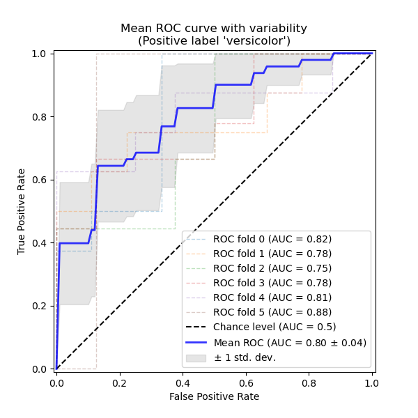
ROC曲線通常在Y軸上具有真正率（true positive rate），在X軸上具有假正率(false positive rate)。這意味著該圖的左上角是“理想”點-誤報率為零，而正誤報率為1。這不是很現實，但這確實意味著，通常來說，曲線下的區域（AUC面積）越大越好。

ROC曲線的“陡峭程度”也很重要，因為理想的是最大程度地提高真正率，同時最小化假正率。

此示例顯示了通過K折交叉驗證創建的不同數據集的ROC曲線。取所有這些曲線，可以計算出曲線下的平均面積，并在訓練集分為不同子集時查看曲線的方差。這大致顯示了分類數據的輸出如何受到訓練數據變化的影響，以及由K折交叉驗證產生的拆分之間的差異如何。

注意：同事也需要查看這些鏈接：sklearn.metrics.roc_auc_score,

sklearn.model_selection.cross_val_score，ROC曲線

輸出：

輸入：

print(__doc__)

import numpy as np
import matplotlib.pyplot as plt

from sklearn import svm, datasets
from sklearn.metrics import auc
from sklearn.metrics import plot_roc_curve
from sklearn.model_selection import StratifiedKFold

# #############################################################################
# 獲取數據

# 導入待處理的數據
iris = datasets.load_iris()
X = iris.data
y = iris.target
X, y = X[y != 2], y[y != 2]
n_samples, n_features = X.shape

# 增加一些噪音特征
random_state = np.random.RandomState(0)
X = np.c_[X, random_state.randn(n_samples, 200 * n_features)]

# #############################################################################
# 分類，并使用ROC曲線分析結果

# 使用交叉驗證運行分類器并繪制ROC曲線
cv = StratifiedKFold(n_splits=6)
classifier = svm.SVC(kernel='linear', probability=True,
                     random_state=random_state)

tprs = []
aucs = []
mean_fpr = np.linspace(0, 1, 100)

fig, ax = plt.subplots()
for i, (train, test) in enumerate(cv.split(X, y)):
    classifier.fit(X[train], y[train])
    viz = plot_roc_curve(classifier, X[test], y[test],
                         name='ROC fold {}'.format(i),
                         alpha=0.3, lw=1, ax=ax)
    interp_tpr = np.interp(mean_fpr, viz.fpr, viz.tpr)
    interp_tpr[0] = 0.0
    tprs.append(interp_tpr)
    aucs.append(viz.roc_auc)

ax.plot([0, 1], [0, 1], linestyle='--', lw=2, color='r',
        label='Chance', alpha=.8)

mean_tpr = np.mean(tprs, axis=0)
mean_tpr[-1] = 1.0
mean_auc = auc(mean_fpr, mean_tpr)
std_auc = np.std(aucs)
ax.plot(mean_fpr, mean_tpr, color='b',
        label=r'Mean ROC (AUC = %0.2f $\pm$ %0.2f)' % (mean_auc, std_auc),
        lw=2, alpha=.8)

std_tpr = np.std(tprs, axis=0)
tprs_upper = np.minimum(mean_tpr + std_tpr, 1)
tprs_lower = np.maximum(mean_tpr - std_tpr, 0)
ax.fill_between(mean_fpr, tprs_lower, tprs_upper, color='grey', alpha=.2,
                label=r'$\pm$ 1 std. dev.')

ax.set(xlim=[-0.05, 1.05], ylim=[-0.05, 1.05],
       title="Receiver operating characteristic example")
ax.legend(loc="lower right")
plt.show()

腳本的總運行時間：（0分鐘0.403秒）