精確度-召回曲線?

本案例用于展示評估分類器輸出質量的精確度-召回曲線。

當樣本的標簽類別非常不平衡時，Precision-Recall是預測是否成功的有用度量。在信息檢索中，精確度是結果相關性的度量，而召回率是返回多少真正相關的結果的度量。

精確度-召回曲線顯示了不同閾值時精度和召回之間的權衡。曲線下的高區域代表高召回率和高精度，其中高精度與低假正率有關，高召回率與低假負率有關。兩者的高分都表明分類器正在返回準確的結果（高精度），并且返回所有正樣本的大部分（高召回率）。

召回率高但精度低的算法會返回許多結果，但是與訓練標簽相比，其大多數預測標簽都不正確。具有高精度但召回率低的系統則相反，返回的結果很少，但是與訓練標簽相比，大多數預測標簽都是正確的。具有高精度和高召回的理想系統將返回許多結果，并且所有結果均正確標記。

精度（）的定義為：真陽性（）的數量超過真陽性的數量加上假陽性（）的數量。

召回（）的定義為：真陽性的數量（）超過真陽性的數量加上假陰性的數量（）。

這些數量還與（）分數相關，該分數定義為精確度和召回的調和平均值。

請注意，精度可能不會隨召回而降低。精度的定義（）表明，降低分類器的閾值可以通過增加返回的結果數來增加分母。如果先前將閾值設置得太高，則新結果可能都是真陽性，這將提高精度。如果先前的閾值大約正確或太低，則進一步降低閾值將引入誤報，從而降低精度。

召回率被定義為，其中不取決于分類器閾值。這意味著降低分類器閾值可能會通過增加真實陽性結果的數量來增加召回率。降低閾值也可能使召回率保持不變，而精度會波動。

可以在繪圖的階梯區域中觀察到召回率與精度之間的關系-在這些步驟的邊緣，閾值的微小變化會顯著降低精度，而召回率只有很小的提高。

平均精度(AP)總結了這樣一個圖，即在每個閾值處獲得的精度的加權平均值，而前一個閾值的召回率增加用作權重：

其中和是第n個閾值的精度和召回率。一對被成為稱為操作點（operating point）。

AP和操作點下的梯形區域（sklearn.metrics.auc）是匯總精確召回曲線的常見方法，可得出不同的結果。在用戶指南中閱讀更多內容。

精確召回曲線通常用于二分類中，以研究分類器的輸出。為了將精確度調用曲線和平均精確度擴展到多類或多標簽分類，必須對輸出進行二值化。每個標簽可以繪制一條曲線，但也可以通過將標簽指示符矩陣的每個元素視為二進制預測（微平均）來繪制精確召回曲線。

注意，請同時查看：sklearn.metrics.average_precision_score,

sklearn.metrics.recall_score, sklearn.metrics.precision_score, sklearn.metrics.f1_score

在二分類情況下

1、創建樣本數據

嘗試區分鳶尾花數據集的前兩個類。

from sklearn import svm, datasets
from sklearn.model_selection import train_test_split
import numpy as np

iris = datasets.load_iris()
X = iris.data
y = iris.target

# 增加噪音特征
random_state = np.random.RandomState(0)
n_samples, n_features = X.shape
X = np.c_[X, random_state.randn(n_samples, 200 * n_features)]

# 限制在前兩個類別上，并且將數據分類為訓練集和測試集
X_train, X_test, y_train, y_test = train_test_split(X[y < 2], y[y < 2],
                                                    test_size=.5,
                                                    random_state=random_state)

# 創建一個簡單的分類器
classifier = svm.LinearSVC(random_state=random_state)
classifier.fit(X_train, y_train)
y_score = classifier.decision_function(X_test)

2、計算平均精確度分數

from sklearn.metrics import average_precision_score
average_precision = average_precision_score(y_test, y_score)

print('Average precision-recall score: {0:0.2f}'.format(
      average_precision))

輸出：

Average precision-recall score: 0.88

3、繪制精確度-召回率曲線

from sklearn.metrics import precision_recall_curve
from sklearn.metrics import plot_precision_recall_curve
import matplotlib.pyplot as plt

disp = plot_precision_recall_curve(classifier, X_test, y_test)
disp.ax_.set_title('2-class Precision-Recall curve: '
                   'AP={0:0.2f}'.format(average_precision))

輸出：

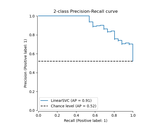
Text(0.5, 1.0, '2-class Precision-Recall curve: AP=0.88')

在多標簽情況下

1、創造多標簽數據，擬合并進行預測

我們創建了一個多標簽數據集，以說明多標簽設置中的精確度-召回率曲線。

from sklearn.preprocessing import label_binarize

# 使用label_binarize讓數據成為類似多標簽的設置
Y = label_binarize(y, classes=[0, 1, 2])
n_classes = Y.shape[1]

# 分割訓練集和測試集
X_train, X_test, Y_train, Y_test = train_test_split(X, Y, test_size=.5,
                                                    random_state=random_state)

# 我們使用OneVsRestClassifier進行多標簽預測
from sklearn.multiclass import OneVsRestClassifier

# 運行分類器
classifier = OneVsRestClassifier(svm.LinearSVC(random_state=random_state))
classifier.fit(X_train, Y_train)
y_score = classifier.decision_function(X_test)

2、多標簽設置中的平均精度得分

from sklearn.metrics import precision_recall_curve
from sklearn.metrics import average_precision_score

# 對每個類別
precision = dict()
recall = dict()
average_precision = dict()
for i in range(n_classes):
    precision[i], recall[i], _ = precision_recall_curve(Y_test[:, i],
                                                        y_score[:, i])
    average_precision[i] = average_precision_score(Y_test[:, i], y_score[:, i])

# 一個"微觀平均": 共同量化所有課程的分數
precision["micro"], recall["micro"], _ = precision_recall_curve(Y_test.ravel(),
    y_score.ravel())
average_precision["micro"] = average_precision_score(Y_test, y_score,
                                                     average="micro")
print('Average precision score, micro-averaged over all classes: {0:0.2f}'
      .format(average_precision["micro"]))

輸出：

Average precision score, micro-averaged over all classes: 0.43

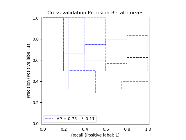
3、繪制微觀平均下的精確召回曲線

plt.figure()
plt.step(recall['micro'], precision['micro'], where='post')

plt.xlabel('Recall')
plt.ylabel('Precision')
plt.ylim([0.0, 1.05])
plt.xlim([0.0, 1.0])
plt.title(
    'Average precision score, micro-averaged over all classes: AP={0:0.2f}'
    .format(average_precision["micro"]))

輸出：

Text(0.5, 1.0, 'Average precision score, micro-averaged over all classes: AP=0.43')

4、為每個類和iso-f1曲線繪制Precision-Recall曲線

from itertools import cycle
# 設置繪圖細節
colors = cycle(['navy', 'turquoise', 'darkorange', 'cornflowerblue', 'teal'])

plt.figure(figsize=(7, 8))
f_scores = np.linspace(0.2, 0.8, num=4)
lines = []
labels = []
for f_score in f_scores:
    x = np.linspace(0.01, 1)
    y = f_score * x / (2 * x - f_score)
    l, = plt.plot(x[y >= 0], y[y >= 0], color='gray', alpha=0.2)
    plt.annotate('f1={0:0.1f}'.format(f_score), xy=(0.9, y[45] + 0.02))

lines.append(l)
labels.append('iso-f1 curves')
l, = plt.plot(recall["micro"], precision["micro"], color='gold', lw=2)
lines.append(l)
labels.append('micro-average Precision-recall (area = {0:0.2f})'
              ''.format(average_precision["micro"]))

for i, color in zip(range(n_classes), colors):
    l, = plt.plot(recall[i], precision[i], color=color, lw=2)
    lines.append(l)
    labels.append('Precision-recall for class {0} (area = {1:0.2f})'
                  ''.format(i, average_precision[i]))

fig = plt.gcf()
fig.subplots_adjust(bottom=0.25)
plt.xlim([0.0, 1.0])
plt.ylim([0.0, 1.05])
plt.xlabel('Recall')
plt.ylabel('Precision')
plt.title('Extension of Precision-Recall curve to multi-class')
plt.legend(lines, labels, loc=(0, -.38), prop=dict(size=14))


plt.show()

輸出：

腳本的總運行時間：（0分鐘0.330秒）