概率校準曲線?

在進行分類時，不僅要預測類標簽，還要預測相關概率。這種概率給了預測某種程度的信心。此示例演示了如何顯示預測概率的校準效果，以及如何校準未校準的分類器。

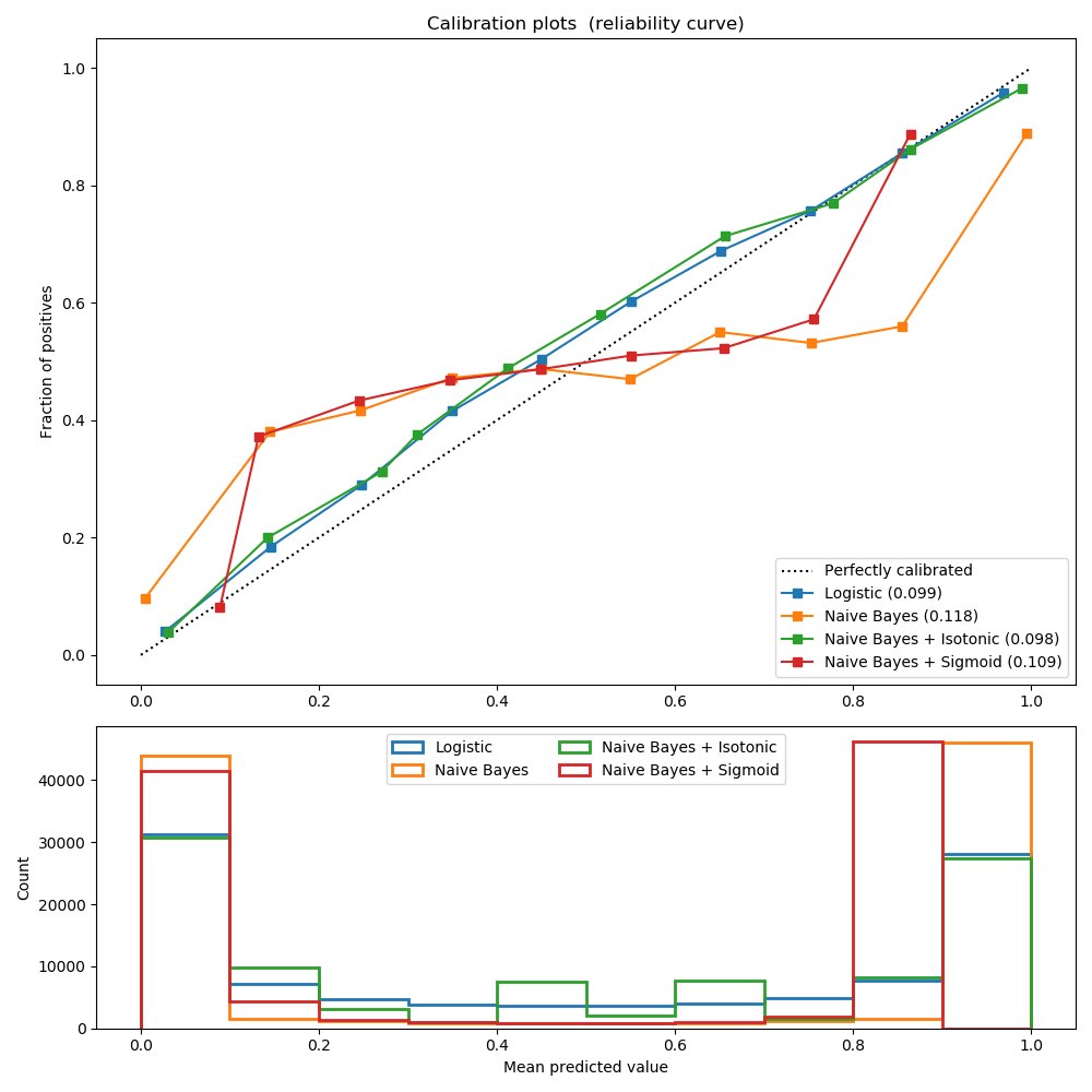
實驗是在一個二分類的人工數據集上進行的，該數據集包含100000個樣本(其中1000個用于模型擬合)，共20個特征。在這20個特性中，只有2個是信息豐富的，10個是冗余的。第一幅圖顯示了通過Logistic回歸、高斯樸素貝葉斯、 isotonic校準的高斯樸素貝葉斯和sigmoid校準的高斯樸素貝葉斯得到的估計概率。校準性能用Brier評分進行評估，在圖例中有報道(越小越好)。這里可以看到，Logistic回歸是很好的校準，而原始高斯樸素貝葉斯表現很差。這是因為冗余特征違背了特征無關的假設，導致分類器過于自信，這可以通過transposed-sigmoid曲線表明。

用 isotonic校準的高斯樸素貝葉斯的概率校準可以解決這一問題，這也可以從對角校準曲線可以看出這一點。sigmoid也略微提高了Brier評分，盡管不如非參數的isotonic回歸那么強。這可以歸因于這樣一個事實：我們有大量的校準數據，以至于可以利用非參數模型的更大的靈活性。

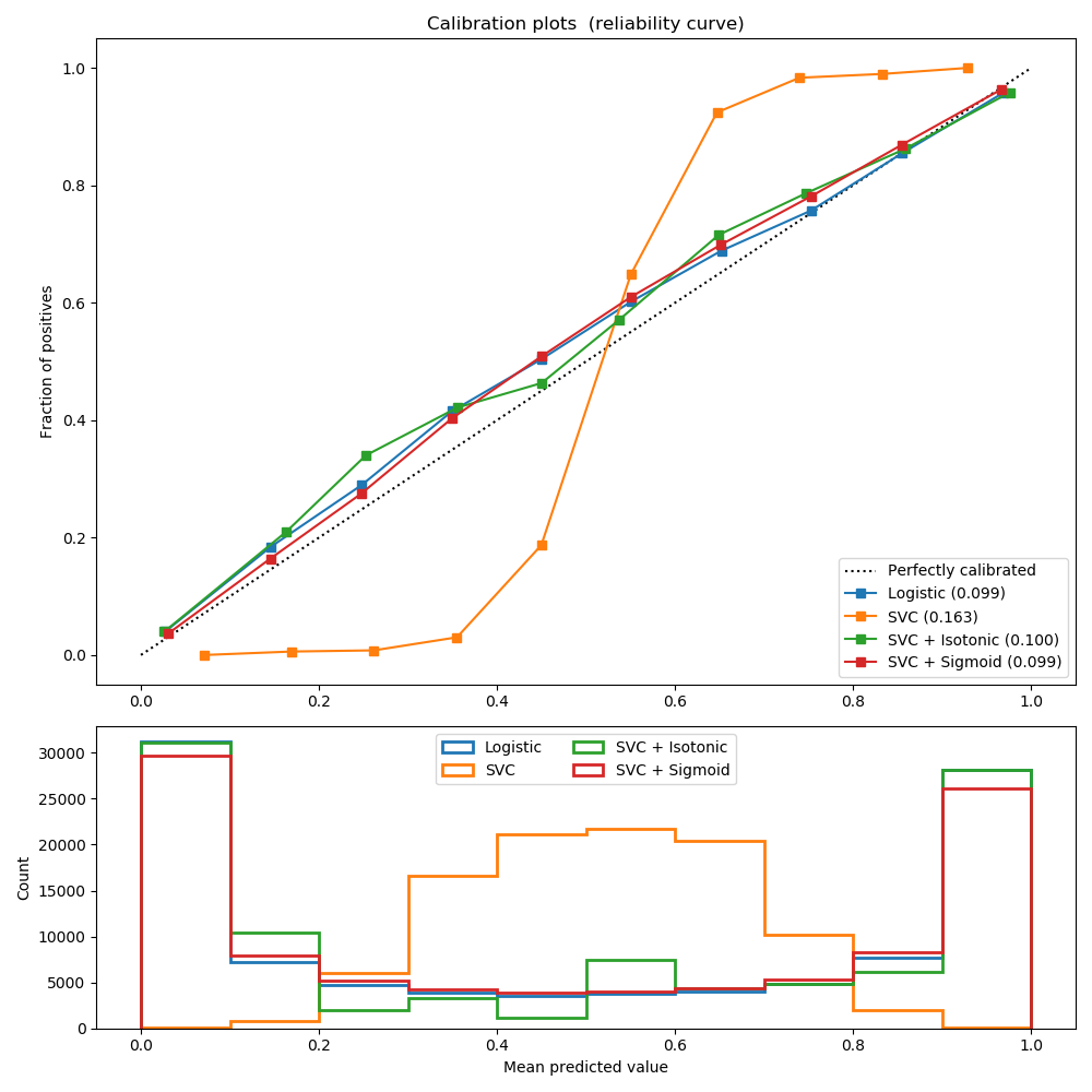
第二個圖顯示了線性支持向量分類器(LinearSVC)的校準曲線。LinearSVC顯示了與高斯樸素貝葉斯相反的行為：校準曲線有一條sigmoid曲線，這是欠自信分類器的典型特征。在LinearSVC的情況下，這是由hinge損失的邊緣特性引起的，這使得模型關注于接近決策邊界的硬樣本(支持向量)。

這兩種校準方法都可以解決這個問題，并得到幾乎相同的結果。這表明，Sigmoid校準可以處理基本分類器的校準曲線為Sigmoid的情況(例如，LinearSVC)，而不能處理transposed-sigmoid(例如，高斯樸素貝葉斯)的情況。

    Logistic:
            Brier: 0.099
            Precision: 0.872
            Recall: 0.851
            F1: 0.862
    
    Naive Bayes:
            Brier: 0.118
            Precision: 0.857
            Recall: 0.876
            F1: 0.867
    
    Naive Bayes + Isotonic:
            Brier: 0.098
            Precision: 0.883
            Recall: 0.836
            F1: 0.859
    
    Naive Bayes + Sigmoid:
            Brier: 0.109
            Precision: 0.861
            Recall: 0.871
            F1: 0.866
    
    Logistic:
            Brier: 0.099
            Precision: 0.872
            Recall: 0.851
            F1: 0.862
    
    SVC:
            Brier: 0.163
            Precision: 0.872
            Recall: 0.852
            F1: 0.862
    
    SVC + Isotonic:
            Brier: 0.100
            Precision: 0.853
            Recall: 0.878
            F1: 0.865
    
    SVC + Sigmoid:
            Brier: 0.099
            Precision: 0.874
            Recall: 0.849
            F1: 0.861

print(__doc__)

# Author: Alexandre Gramfort <alexandre.gramfort@telecom-paristech.fr>
#         Jan Hendrik Metzen <jhm@informatik.uni-bremen.de>
# License: BSD Style.

import matplotlib.pyplot as plt

from sklearn import datasets
from sklearn.naive_bayes import GaussianNB
from sklearn.svm import LinearSVC
from sklearn.linear_model import LogisticRegression
from sklearn.metrics import (brier_score_loss, precision_score, recall_score,
                             f1_score)
from sklearn.calibration import CalibratedClassifierCV, calibration_curve
from sklearn.model_selection import train_test_split


# Create dataset of classification task with many redundant and few
# informative features
X, y = datasets.make_classification(n_samples=100000, n_features=20,
                                    n_informative=2, n_redundant=10,
                                    random_state=42)

X_train, X_test, y_train, y_test = train_test_split(X, y, test_size=0.99,
                                                    random_state=42)


def plot_calibration_curve(est, name, fig_index):
    """Plot calibration curve for est w/o and with calibration. """
    # Calibrated with isotonic calibration
    isotonic = CalibratedClassifierCV(est, cv=2, method='isotonic')

    # Calibrated with sigmoid calibration
    sigmoid = CalibratedClassifierCV(est, cv=2, method='sigmoid')

    # Logistic regression with no calibration as baseline
    lr = LogisticRegression(C=1.)

    fig = plt.figure(fig_index, figsize=(10, 10))
    ax1 = plt.subplot2grid((3, 1), (0, 0), rowspan=2)
    ax2 = plt.subplot2grid((3, 1), (2, 0))

    ax1.plot([0, 1], [0, 1], "k:", label="Perfectly calibrated")
    for clf, name in [(lr, 'Logistic'),
                      (est, name),
                      (isotonic, name + ' + Isotonic'),
                      (sigmoid, name + ' + Sigmoid')]:
        clf.fit(X_train, y_train)
        y_pred = clf.predict(X_test)
        if hasattr(clf, "predict_proba"):
            prob_pos = clf.predict_proba(X_test)[:, 1]
        else:  # use decision function
            prob_pos = clf.decision_function(X_test)
            prob_pos = \
                (prob_pos - prob_pos.min()) / (prob_pos.max() - prob_pos.min())

        clf_score = brier_score_loss(y_test, prob_pos, pos_label=y.max())
        print("%s:" % name)
        print("\tBrier: %1.3f" % (clf_score))
        print("\tPrecision: %1.3f" % precision_score(y_test, y_pred))
        print("\tRecall: %1.3f" % recall_score(y_test, y_pred))
        print("\tF1: %1.3f\n" % f1_score(y_test, y_pred))

        fraction_of_positives, mean_predicted_value = \
            calibration_curve(y_test, prob_pos, n_bins=10)

        ax1.plot(mean_predicted_value, fraction_of_positives, "s-",
                 label="%s (%1.3f)" % (name, clf_score))

        ax2.hist(prob_pos, range=(0, 1), bins=10, label=name,
                 histtype="step", lw=2)

    ax1.set_ylabel("Fraction of positives")
    ax1.set_ylim([-0.05, 1.05])
    ax1.legend(loc="lower right")
    ax1.set_title('Calibration plots  (reliability curve)')

    ax2.set_xlabel("Mean predicted value")
    ax2.set_ylabel("Count")
    ax2.legend(loc="upper center", ncol=2)

    plt.tight_layout()

# Plot calibration curve for Gaussian Naive Bayes
plot_calibration_curve(GaussianNB(), "Naive Bayes", 1)

# Plot calibration curve for Linear SVC
plot_calibration_curve(LinearSVC(max_iter=10000), "SVC", 2)

plt.show()

腳本的總運行時間：(0分2.485秒)