分類器的概率校準?
在執行分類時,不僅要預測類標簽,還要預測相關的概率。這個概率給了你對這個預測的某種信心。然而,并不是所有的分類器都能提供精確的概率,有些是過于自信,而另一些則是不夠自信。因此,作為后處理,單獨的校準預測概率通常是可取的。此示例說明了兩種不同的校準方法,并使用Brier評分評估返回概率的質量。(看 https://en.wikipedia.org/wiki/Brier_score)
比較了使用高斯樸素貝葉斯分類器進行不校準、sigmoid校準和非參數 isotonic 校準的估計概率。可以觀察到,只有非參數模型能夠提供概率校準,對于大多數屬于具有異質標簽的中間聚類的樣本,返回的概率接近預期的0.5。這導致Brier評分顯著提高。
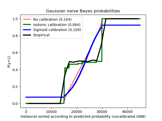
Brier scores: (the smaller the better)
No calibration: 0.104
With isotonic calibration: 0.084
With sigmoid calibration: 0.109
print(__doc__)
# Author: Mathieu Blondel <mathieu@mblondel.org>
# Alexandre Gramfort <alexandre.gramfort@telecom-paristech.fr>
# Balazs Kegl <balazs.kegl@gmail.com>
# Jan Hendrik Metzen <jhm@informatik.uni-bremen.de>
# License: BSD Style.
import numpy as np
import matplotlib.pyplot as plt
from matplotlib import cm
from sklearn.datasets import make_blobs
from sklearn.naive_bayes import GaussianNB
from sklearn.metrics import brier_score_loss
from sklearn.calibration import CalibratedClassifierCV
from sklearn.model_selection import train_test_split
n_samples = 50000
n_bins = 3 # use 3 bins for calibration_curve as we have 3 clusters here
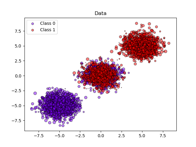
# Generate 3 blobs with 2 classes where the second blob contains
# half positive samples and half negative samples. Probability in this
# blob is therefore 0.5.
centers = [(-5, -5), (0, 0), (5, 5)]
X, y = make_blobs(n_samples=n_samples, centers=centers, shuffle=False,
random_state=42)
y[:n_samples // 2] = 0
y[n_samples // 2:] = 1
sample_weight = np.random.RandomState(42).rand(y.shape[0])
# split train, test for calibration
X_train, X_test, y_train, y_test, sw_train, sw_test = \
train_test_split(X, y, sample_weight, test_size=0.9, random_state=42)
# Gaussian Naive-Bayes with no calibration
clf = GaussianNB()
clf.fit(X_train, y_train) # GaussianNB itself does not support sample-weights
prob_pos_clf = clf.predict_proba(X_test)[:, 1]
# Gaussian Naive-Bayes with isotonic calibration
clf_isotonic = CalibratedClassifierCV(clf, cv=2, method='isotonic')
clf_isotonic.fit(X_train, y_train, sample_weight=sw_train)
prob_pos_isotonic = clf_isotonic.predict_proba(X_test)[:, 1]
# Gaussian Naive-Bayes with sigmoid calibration
clf_sigmoid = CalibratedClassifierCV(clf, cv=2, method='sigmoid')
clf_sigmoid.fit(X_train, y_train, sample_weight=sw_train)
prob_pos_sigmoid = clf_sigmoid.predict_proba(X_test)[:, 1]
print("Brier scores: (the smaller the better)")
clf_score = brier_score_loss(y_test, prob_pos_clf, sample_weight=sw_test)
print("No calibration: %1.3f" % clf_score)
clf_isotonic_score = brier_score_loss(y_test, prob_pos_isotonic,
sample_weight=sw_test)
print("With isotonic calibration: %1.3f" % clf_isotonic_score)
clf_sigmoid_score = brier_score_loss(y_test, prob_pos_sigmoid,
sample_weight=sw_test)
print("With sigmoid calibration: %1.3f" % clf_sigmoid_score)
# #############################################################################
# Plot the data and the predicted probabilities
plt.figure()
y_unique = np.unique(y)
colors = cm.rainbow(np.linspace(0.0, 1.0, y_unique.size))
for this_y, color in zip(y_unique, colors):
this_X = X_train[y_train == this_y]
this_sw = sw_train[y_train == this_y]
plt.scatter(this_X[:, 0], this_X[:, 1], s=this_sw * 50,
c=color[np.newaxis, :],
alpha=0.5, edgecolor='k',
label="Class %s" % this_y)
plt.legend(loc="best")
plt.title("Data")
plt.figure()
order = np.lexsort((prob_pos_clf, ))
plt.plot(prob_pos_clf[order], 'r', label='No calibration (%1.3f)' % clf_score)
plt.plot(prob_pos_isotonic[order], 'g', linewidth=3,
label='Isotonic calibration (%1.3f)' % clf_isotonic_score)
plt.plot(prob_pos_sigmoid[order], 'b', linewidth=3,
label='Sigmoid calibration (%1.3f)' % clf_sigmoid_score)
plt.plot(np.linspace(0, y_test.size, 51)[1::2],
y_test[order].reshape(25, -1).mean(1),
'k', linewidth=3, label=r'Empirical')
plt.ylim([-0.05, 1.05])
plt.xlabel("Instances sorted according to predicted probability "
"(uncalibrated GNB)")
plt.ylabel("P(y=1)")
plt.legend(loc="upper left")
plt.title("Gaussian naive Bayes probabilities")
plt.show()
腳本的總運行時間:(0分0.459秒)