sklearn.decomposition.NMF?
class sklearn.decomposition.NMF(n_components=None, *, init=None, solver='cd', beta_loss='frobenius', tol=0.0001, max_iter=200, random_state=None, alpha=0.0, l1_ratio=0.0, verbose=0, shuffle=False)
非負矩陣分解
找出兩個非負矩陣(W, H),它們的乘積近似于非負矩陣x。這種分解可以用于降維、源分離或主題提取。
目標函數為:
0.5 * ||X - WH||_Fro^2
+ alpha * l1_ratio * ||vec(W)||_1
+ alpha * l1_ratio * ||vec(H)||_1
+ 0.5 * alpha * (1 - l1_ratio) * ||W||_Fro^2
+ 0.5 * alpha * (1 - l1_ratio) * ||H||_Fro^2
Where:
||A||_Fro^2 = \sum_{i,j} A_{ij}^2 (Frobenius norm)
||vec(A)||_1 = \sum_{i,j} abs(A_{ij}) (Elementwise L1 norm)
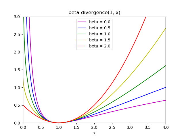
對于乘更新(' mu ')求解器,通過改變參數beta_loss,可以將Frobenius范數(0.5 * ||X - WH||_Fro^2)變為另一個散度損失。
通過W和H的交替最小化來最小化目標函數。
在用戶指南中閱讀更多內容
新版本 0.18 。
| 參數 | 說明 |
|---|---|
| n_components | int or None 樣本的數量,如果沒有設置n_components,則保留所有特性。 |
| init | None / ‘random’ / ‘nndsvd’ / ‘nndsvda’ / ‘nndsvdar’ / ‘custom’ 用于初始化過程的方法。默認值:None。有效的選項: None: ‘nndsvd’ if n_components <= min(n_samples, n_features) 否則隨機。 ‘random’: non-negative random matrices, scaled with: sqrt(X.mean() / n_components) ‘nndsvd’: Nonnegative Double Singular Value Decomposition (NNDSVD) 初始化 (better for sparseness) ‘nndsvda’: NNDSVD with zeros filled with the average of X (better when sparsity is not desired) ‘nndsvdar’: NNDSVD with zeros filled with small random values (當不需要稀疏性時,通常更快,更不精確的NNDSVDa替代方案) ‘custom’: 使用自定義矩陣W和H |
| solver | 'cd'/'mu' “cd”是一個坐標下降求解器。' mu '是一個乘法更新求解器。 新版本0.17:坐標下降求解器。 版本0.19中的新版本:乘法更新求解器。 |
| beta_loss | float or string, default ‘frobenius’ 字符串必須是{' frobenius ', ' kullback-leibler ', ' itakura-saito '}。為了使散度最小,測量X和點積WH之間的距離。注意,與“frobenius”(或2)和“kullback-leibler”(或1)不同的值會導致匹配速度明顯較慢。注意,對于beta_loss <= 0(或' itakura-saito '),輸入矩陣X不能包含0。只在求解器中使用。 新版本為0.19。 |
| tol | float, default: 1e-4 停止條件的容忍度。 |
| max_iter | integer, default: 200 超時前的最大迭代次數。 |
| random_state | int, RandomState instance, default=None 用于初始化(當 init== ' nndsvdar '或' random '),并在坐標下降。在多個函數調用中傳遞可重復的結果。詳見術語表。。 |
| alpha | double, default: 0. 乘正則化項的常數。將它設為0,這樣就沒有正則化。 在0.17版本中新增:用于坐標下降求解器的alpha。 |
| l1_ratio | double, default: 0. 正則化混合參數,0 <= l1_ratio <= 1。對于l1_ratio = 0,罰分為元素L2罰分(又名Frobenius Norm)。對于l1_ratio = 1,它是元素上的L1懲罰。對于0 < l1_ratio < 1,懲罰為L1和L2的組合。 在0.17版本中新增:在坐標下降求解器中使用正則化參數l1_ratio。 |
| verbose | bool, default=False 是否冗長。 |
| shuffle | boolean, default: False If true, randomize the order of coordinates in the CD solver. |
| 屬性 | 說明 |
|---|---|
| components_ | array, [n_components, n_features] 分解矩陣,有時稱為“字典”。 |
| n_components_ | integer 組件的數量。如果給定n_components參數,則它與n_components參數相同。否則,它將與特性的數量相同。 |
| reconstruction_err_ | number 訓練數據X與擬合模型重建數據WH之間的矩陣差(或貝塔散度)的Frobenius范數。 |
| n_iter_ | int 實際迭代次數。 |
參考文獻
Cichocki, Andrzej, and P. H. A. N. Anh-Huy. “Fast local algorithms for large scale nonnegative matrix and tensor factorizations.” IEICE transactions on fundamentals of electronics, communications and computer sciences 92.3: 708-721, 2009.
Fevotte, C., & Idier, J. (2011). Algorithms for nonnegative matrix factorization with the beta-divergence. Neural Computation, 23(9).
示例
>>> import numpy as np
>>> X = np.array([[1, 1], [2, 1], [3, 1.2], [4, 1], [5, 0.8], [6, 1]])
>>> from sklearn.decomposition import NMF
>>> model = NMF(n_components=2, init='random', random_state=0)
>>> W = model.fit_transform(X)
>>> H = model.components_
方法
| 方法 | 說明 |
|---|---|
fit(X[, y]) |
學習數據X的NMF模型。 |
fit_transform(X[, y, W, H]) |
學習數據X的NMF模型并返回轉換后的數據。 |
get_params([deep]) |
獲取這個估計器的參數。 |
inverse_transform(W) |
將數據轉換回其原始空間。 |
set_params(**params) |
設置這個估計器的參數。 |
transform(X) |
根據擬合的NMF模型對數據X進行變換 |
__init__(n_components=None, *, init=None, solver='cd', beta_loss='frobenius', tol=0.0001, max_iter=200, random_state=None, alpha=0.0, l1_ratio=0.0, verbose=0, shuffle=False)
初始化self. See 請參閱help(type(self))以獲得準確的說明。
fit(X, y=None, **params)
學習數據X的NMF模型。
| 參數 | 說明 |
|---|---|
| X | {array-like, sparse matrix}, shape (n_samples, n_features) 待分解的數據矩陣 |
| y | Ignored |
| 返回值 | 說明 |
|---|---|
| self | - |
fit_transform(X, y=None, W=None, H=None)
學習數據X的NMF模型并返回轉換后的數據。
這比先調用fit再進行轉換更有效。
| 參數 | 說明 |
|---|---|
| X | {array-like, sparse matrix, dataframe} of shape (n_samples, n_features) 待分解的數據矩陣 |
| y | Ignored |
| W | array-like, shape (n_samples, n_components) 如果 init= ' custom ',則使用它作為解決方案的初始猜測。 |
| H | array-like, shape (n_components, n_features) 如果 init= ' custom ',則使用它作為解決方案的初始猜測。 |
| 返回值 | 說明 |
|---|---|
| W | array, shape (n_samples, n_components) 轉換數據。 |
get_params(deep=True)
獲取這個估計器的參數。
| 參數 | 說明 |
|---|---|
| deep | bool, default=True 如果為True,則將返回此估計器的參數和所包含的作為估計器的子對象。 |
| 返回值 | 說明 |
|---|---|
| X_new | ndarray array of shape (n_samples, n_features_new) 轉換的數組 |
inverse_transform(W)
將數據轉換回其原始空間。
| 參數 | 說明 |
|---|---|
| W | {array-like, sparse matrix}, shape (n_samples, n_components) 轉換后的數據矩陣 |
| 返回值 | 說明 |
|---|---|
| X | {array-like, sparse matrix}, shape (n_samples, n_features) 原始形狀的數據矩陣 新版本 0.18 。 |
set_params(*params)
設置這個估計器的參數。
該方法適用于簡單估計量和嵌套對象(如pipelines)。后者具有形式為<component>_<parameter>的參數,這樣就讓更新嵌套對象的每個組件成為了可能。
| 參數 | 說明 |
|---|---|
| **params | dict 估計參數。 |
| 返回值 | 說明 |
|---|---|
| self | object 估計參數。 |
transform(X)
根據擬合的NMF模型對數據X進行變換
| 參數 | 說明 |
|---|---|
| X | {array-like, sparse matrix}, shape (n_samples, n_features) 模型需要轉換的數據矩陣 |
| 返回值 | 說明 |
|---|---|
| W | array, shape (n_samples, n_components) 轉換后的數據 |