sklearn.decomposition.PCA?
class sklearn.decomposition.PCA(n_components=None, *, copy=True, whiten=False, svd_solver='auto', tol=0.0, iterated_power='auto', random_state=None)
主成分分析(PCA)。
利用數據的奇異值分解將其投射到較低維空間的線性降維。在應用SVD之前,輸入數據是居中的,但沒有針對每個特征進行縮放。
根據輸入數據的形狀和提取的分量的數量,它使用LAPACK實現的完整SVD或隨機截斷的SVD Halko et al. 2009的方法。
它也可以使用scipy.sparse。linalg ARPACK的截斷SVD實現。
請注意,這個類不支持稀疏輸入。請參閱TruncatedSVD了解稀疏數據的替代方法。
在用戶指南中閱讀更多內容
| 參數 | 說明 |
|---|---|
| n_components | int, float, None or str 要保存的樣本數量。如果沒有設置n_components,則保留所有樣本: n_components == min(n_samples, n_features) 如果 n_components == 'mle' and svd_solver == 'full', 則使用Minka’s MLE 來猜測維數. 使用n_components == 'mle' 講把 svd_solver == 'auto' 解釋為 svd_solver == 'full'.如果 0 < n_components < 1 and svd_solver == 'full', 則選擇樣本的數量,以便需要解釋的方差量大于n_components指定的百分比。如果 svd_solver == 'arpack', 則組件的數量必須嚴格小于n_features和n_samples的最小值。因此,None case的結果是: n_components == min(n_samples, n_features) - 1 |
| copy | bool, default=True 如果為False,傳遞給fit的數據將被覆蓋,運行fit(X).transform(X)將不會產生預期的結果,使用fit_transform(X)代替。 |
| whiten | bool, optional (default False) 當為真(默認為假)時,components_向量乘以n_samples的平方根,然后除以奇異值,以確保輸出與單位分量方差不相關。 白化將從轉換信號中去除一些信息(組件的相對方差尺度),但有時可以通過使下游估計器的數據尊重一些硬連接的假設來提高其預測精度。 |
| svd_solver | str {‘auto’, ‘full’, ‘arpack’, ‘randomized’} If auto : 根據基于X的默認策略選擇求解器。shape和n_components:如果輸入數據大于500x500,并且要提取的組件數量小于數據最小維數的80%,那么就啟用了更有效的“隨機化”方法。否則,精確的完整SVD將被計算,然后選擇性地截斷。 If full : 通過scipy.linalg調用標準的LAPACK求解器運行精確的全SVD。svd和選擇組件的后處理 If arpack : 通過sci . sparsee .linalg.svds調用ARPACK求解器來運行截斷為n_components的SVD。它嚴格要求0 < n_components < min(X.shape) If randomized : 使用Halko等的方法進行隨機化SVD。 |
| tol | float >= 0, optional (default .0) svd_solver == ' arpack '計算的奇異值的容忍度。 新版本0.18.0。 |
| iterated_power | int >= 0, or ‘auto’, (default ‘auto’) svd_solver計算的冪次法的迭代次數== ' random '。 新版本0.18.0。 |
| random_state | int, RandomState instance, default=None 當 svd_solver == ' arpack '或' randomver '時使用。在多個函數調用中傳遞可重復的結果。詳見術語表。新版本0.18.0。 |
| 屬性 | 說明 |
|---|---|
| components_ | array, shape (n_components, n_features) 特征空間的主軸,表示數據中方差最大的方向。樣本按 explained_variance_排序。 |
| explained_variance_ | array, shape (n_components,) 所選擇的每個分量所解釋的方差量。 等于X的協方差矩陣的n個最大特征值。 新版本0.18。 |
| explained_variance_ratio_ | array, shape (n_components,) 所選擇的每個組成部分所解釋的方差百分比。 如果沒有設置 n_components,那么將存儲所有組件,并且比率的總和等于1.0。 |
| singular_values_ | array, shape (n_components,) 對應于每個選定分量的奇異值。奇異值等于低維空間中 n_component變量的2-范數。新版本為0.19。 |
| mean_ | array, shape (n_features,) 每個特征的經驗平均數,從訓練集估計。 等于 X.mean(axis=0). |
| n_components_ | int 估計的組件數量。當n_components設置為' mle '或0到1之間的數字(with svd_solver == ‘full’)時,該數字是從輸入數據估計的。否則等于參數 n_components,或者如果n_components為None,則等于n_features和n_samples的較小值。 |
| n_features_ | int 訓練數據中的特征數。 |
| n_samples_ | int 訓練數據中的樣本數。 |
| noise_variance_ | float 根據Tipping和Bishop 1999年的概率PCA模型估計的噪聲協方差。參見C. Bishop的“模式識別和機器學習”,12.2.1頁,574或http://www.miketipping.com/papers/met-mppca.pdf。需要計算估計數據協方差和樣本評分。 等于X的協方差矩陣的最小特征值 (min(n_features, n_samples) - n_components)的平均值。 |
另見:
Kernel Principal Component Analysis.
Sparse Principal Component Analysis.
Dimensionality reduction using truncated SVD.
Incremental Principal Component Analysis.
參考資料:
For n_components == ‘mle’, this class uses the method of Minka, T. P. “Automatic choice of dimensionality for PCA”. In NIPS, pp. 598-604
Implements the probabilistic PCA model from: Tipping, M. E., and Bishop, C. M. (1999). “Probabilistic principal component analysis”. Journal of the Royal Statistical Society: Series B (Statistical Methodology), 61(3), 611-622. via the score and score_samples methods. See http://www.miketipping.com/papers/met-mppca.pdf
For svd_solver == ‘arpack’, refer to scipy.sparse.linalg.svds.
For svd_solver == ‘randomized’, see: Halko, N., Martinsson, P. G., and Tropp, J. A. (2011). “Finding structure with randomness: Probabilistic algorithms for constructing approximate matrix decompositions”. SIAM review, 53(2), 217-288. and also Martinsson, P. G., Rokhlin, V., and Tygert, M. (2011). “A randomized algorithm for the decomposition of matrices”. Applied and Computational Harmonic Analysis, 30(1), 47-68.
>>> import numpy as np
>>> from sklearn.decomposition import PCA
>>> X = np.array([[-1, -1], [-2, -1], [-3, -2], [1, 1], [2, 1], [3, 2]])
>>> pca = PCA(n_components=2)
>>> pca.fit(X)
PCA(n_components=2)
>>> print(pca.explained_variance_ratio_)
[0.9924... 0.0075...]
>>> print(pca.singular_values_)
[6.30061... 0.54980...]
>>>
>>> pca = PCA(n_components=2, svd_solver='full')
>>> pca.fit(X)
PCA(n_components=2, svd_solver='full')
>>> print(pca.explained_variance_ratio_)
[0.9924... 0.00755...]
>>> print(pca.singular_values_)
[6.30061... 0.54980...]
>>>
>>> pca = PCA(n_components=1, svd_solver='arpack')
>>> pca.fit(X)
PCA(n_components=1, svd_solver='arpack')
>>> print(pca.explained_variance_ratio_)
[0.99244...]
>>> print(pca.singular_values_)
[6.30061...]
方法
| 方法 | 說明 |
|---|---|
fit(X[, y]) |
用X擬合模型。 |
fit_transform(X[, y]) |
用X擬合模型,對X進行降維。 |
get_covariance() |
用生成模型計算數據協方差。 |
get_params([deep]) |
獲取這個估計器的參數。 |
get_precision() |
利用生成模型計算數據精度矩陣。 |
inverse_transform(X) |
將數據轉換回其原始空間。 |
score(X[, y]) |
返回所有樣本的平均對數似然值。 |
score_samples(X) |
返回每個樣本的對數似然值。 |
set_params(**params) |
設置這個估計器的參數。 |
transform(X) |
對X應用維數約簡。 |
__init__(n_components=None, *, copy=True, whiten=False, svd_solver='auto', tol=0.0, iterated_power='auto', random_state=None)
初始化self. See 請參閱help(type(self))以獲得準確的說明。
fit(X, y=None)
用X擬合模型,對X進行降維。
| 參數 | 說明 |
|---|---|
| X | array-like, shape (n_samples, n_features) 訓練向量,其中樣本數量中的n_samples和n_features為feature的數量。 |
| y | Ignored |
| 返回值 | 說明 |
|---|---|
| X_new | ndarray array of shape (n_samples, n_features_new) 轉換的數組 |
注意:
此方法返回一個按fortran順序排列的數組。要將其轉換為c順序數組,請使用“np. ascontinuity array”。
get_covariance()
用生成模型計算數據協方差。
cov = components_.T * S**2 * components_ + sigma2 * eye(n_features) S**2包含被解釋的方差,sigma2包含噪聲方差。
| 返回值 | 說明 |
|---|---|
| cov | array, shape=(n_features, n_features) 數據的估計協方差。 |
get_params(deep=True)
利用生成模型計算數據精度矩陣。
等于協方差的逆,但為了效率,用矩陣逆引理計算。
| 返回值 | 說明 |
|---|---|
| precision | **array, shape=(n_features, n_features)**** 數據的估計精度。 |
inverse_transform(X)
將數據轉換回其原始空間。
換句話說,返回一個轉換為X的輸入X_original。
| 參數 | 說明 |
|---|---|
| X | array-like, shape (n_samples, n_components) 新數據,其中n_samples是樣本的數量,n_components是組件的數量。 |
| 返回值 | 說明 |
|---|---|
| X_original array-like, shape (n_samples, n_features) | 略 |
注意:
如果啟用了白化,inverse_transform將計算精確的反運算,其中包括反向白化。
score(X, y=None)
返回所有樣本的平均對數似然值。
另見:
“Pattern Recognition and Machine Learning” by C. Bishop, 12.2.1 p. 574 or http://www.miketipping.com/papers/met-mppca.pdf
| 參數 | 說明 |
|---|---|
| X | array-like, shape (n_samples, n_features) 數據 |
| y | None 忽略的變量。 |
| 返回值 | 說明書 |
|---|---|
| II | float 樣本在當前模型下的對數似然平均數。 |
score_samples(X)
返回每個樣本的對數似然值。
另見:
“Pattern Recognition and Machine Learning” by C. Bishop, 12.2.1 p. 574 or http://www.miketipping.com/papers/met-mppca.pdf
| 參數 | 說明 |
|---|---|
| X | array-like, shape (n_samples, n_features) 數據 |
| 返回值 | 說明書 |
|---|---|
| II | array, shape (n_samples,) 樣本在當前模型下的對數似然平均數。 |
set_params(**params)
設置這個估計器的參數。
該方法適用于簡單估計量和嵌套對象。后者具有形式為<component>_<parameter>的參數,這樣就讓更新嵌套對象的每個組件成為了可能。
| 參數 | 說明 |
|---|---|
| **params | dict 估計器參數。 |
| 返回值 | 說明書 |
|---|---|
| self | object 估計器參數。 |
transform(X)
對X應用維數約簡。
X被投影到之前從訓練集中提取的第一個主成分上。
| 參數 | 說明 |
|---|---|
| X | array-like, shape (n_samples, n_features) 新數據,其中n_samples為樣本數量,n_features為特征數量。 |
| 返回值 | 說明書 |
|---|---|
| X_new | array-like, shape (n_samples, n_components) |
示例:
>>> import numpy as np
>>> from sklearn.decomposition import IncrementalPCA
>>> X = np.array([[-1, -1], [-2, -1], [-3, -2], [1, 1], [2, 1], [3, 2]])
>>> ipca = IncrementalPCA(n_components=2, batch_size=3)
>>> ipca.fit(X)
IncrementalPCA(batch_size=3, n_components=2)
>>> ipca.transform(X) # doctest: +SKIP