sklearn.decomposition.TruncatedSVD?
class sklearn.decomposition.TruncatedSVD(n_components=2, *, algorithm='randomized', n_iter=5, random_state=None, tol=0.0)
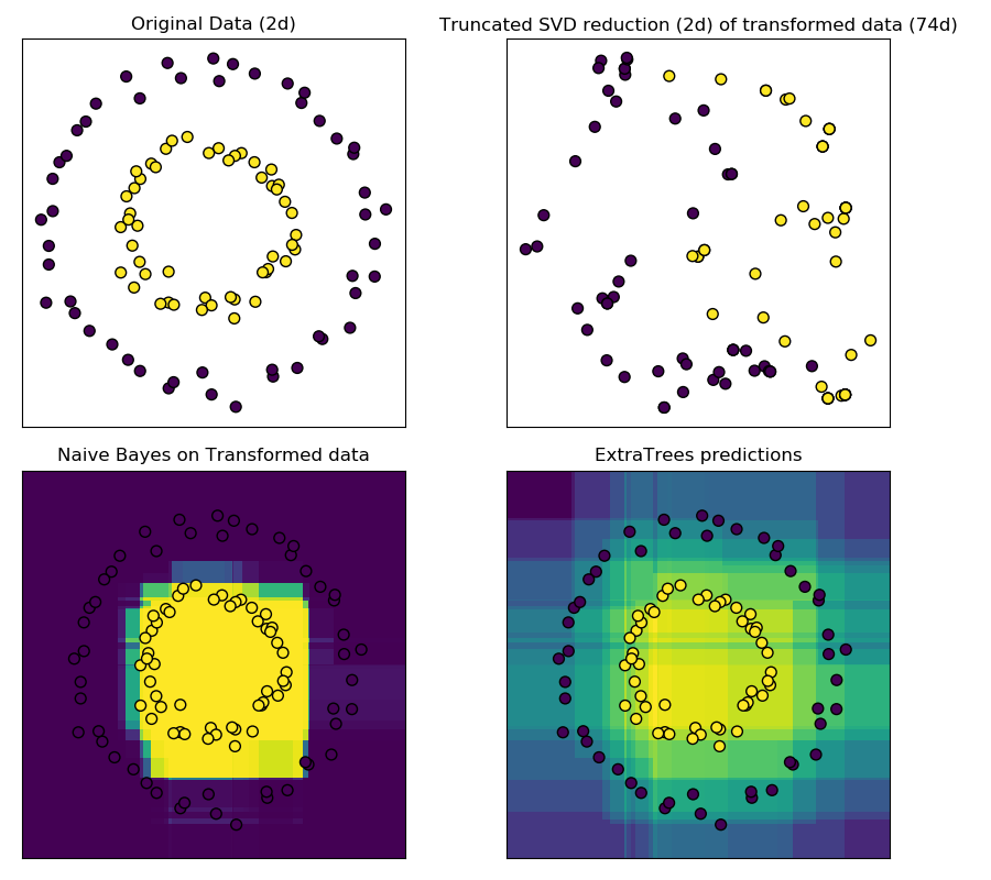
使用截斷SVD(即LSA)降維。
該變壓器采用截斷奇異值分解(SVD)進行線性降維。與主成分分析相反,該估計器在計算奇異值分解前不集中數據。這意味著它可以有效地處理稀疏矩陣。
特別地,截斷的SVD適用于由sklearn.feature_extraction.text中的矢量器返回的term count/tf-idf矩陣。在這種情況下,它被稱為潛在語義分析(LSA)。
該估計器支持兩種算法:一種是快速隨機SVD求解器,另一種是在X * X.T or X.T * X上使用ARPACK作為特征求解器的“天真”算法.X * X.T or X.T * X哪個效率更高。
在用戶指南中閱讀更多內容
| 參數 | 說明 |
|---|---|
| n_components | int, default = 2 輸出數據的期望維數。必須嚴格小于特性的數量。默認值對可視化很有用。對于LSA,建議值為100。 |
| algorithm | string, default = “randomized” SVD求解器使用。或者用“arpack”表示SciPy中的arpack包裝(SciPy .sparse.linalg.svds),或者用“random”表示由Halko(2009)提出的隨機算法。 |
| n_iter | int, optional (default 5) 隨機SVD求解器的迭代次數。ARPACK沒有使用。默認值比 randomized_svd中的默認值大,用于處理可能有較大的緩慢衰減頻譜的稀疏矩陣。 |
| random_state | int, RandomState instance, default=None 用于隨機svd。在多個函數調用中傳遞可重復的結果。詳見術語表。 |
| tol | float, optional 對ARPACK的容忍度。0表示機器精度。隨機SVD求解器忽略。 |
| 屬性 | 說明 |
|---|---|
| components_ | array, shape (n_components, n_features) |
| explained_variance_ | array, shape (n_components,) 訓練樣本的方差由投影轉換到每個分量。 |
| explained_variance_ratio_ | array, shape (n_components,) 所選擇的每個組成部分所解釋的方差百分比。 |
| singular_values_ | array, shape (n_components,) 對應于每個選定分量的奇異值。奇異值等于低維空間中 n_component變量的2-范數。 |
另見:
注意:
SVD有一個叫做“符號不確定性”的問題,這意味著 components_ 的符號和transform的輸出依賴于算法和隨機狀態。要解決這個問題,只需將該類的實例與數據匹配一次,然后保留該實例來執行轉換。
參考文獻:
Finding structure with randomness: Stochastic algorithms for constructing approximate matrix decompositions Halko, et al., 2009 (arXiv:909) https://arxiv.org/pdf/0909.4061.pdf
示例:
>>> from sklearn.decomposition import TruncatedSVD
>>> from scipy.sparse import random as sparse_random
>>> from sklearn.random_projection import sparse_random_matrix
>>> X = sparse_random(100, 100, density=0.01, format='csr',
...                   random_state=42)
>>> svd = TruncatedSVD(n_components=5, n_iter=7, random_state=42)
>>> svd.fit(X)
TruncatedSVD(n_components=5, n_iter=7, random_state=42)
>>> print(svd.explained_variance_ratio_)
[0.0646... 0.0633... 0.0639... 0.0535... 0.0406...]
>>> print(svd.explained_variance_ratio_.sum())
0.286...
>>> print(svd.singular_values_)
[1.553... 1.512...  1.510... 1.370... 1.199...]
方法:
| 方法 | 說明 |
|---|---|
fit(X[, y]) |
在訓練數據X上擬合LSI模型。 |
fit_transform(X[, y]) |
將LSI模型擬合到X上,對X進行降維。 |
get_params([deep]) |
獲取這個估計器的參數。 |
inverse_transform(X) |
將X變換回原來的空間。 |
set_params(**params) |
設置這個估計器的參數。 |
transform(X) |
對X進行降維。 |
__init__(n_components=2, *, algorithm='randomized', n_iter=5, random_state=None, tol=0.0)
初始化self. See 請參閱help(type(self))以獲得準確的說明。
fit(X, y=None)[source]
在訓練數據X上擬合LSI模型。
| 參數 | 說明 |
|---|---|
| X | array-like, shape (n_samples, n_features) 訓練向量,其中樣本數量中的n_samples和n_features為feature的數量。 |
| y | Ignored |
| 返回值 | 說明書 |
|---|---|
| self | object 返回transformer對象。 |
fit_transform(X, y=None)
將LSI模型擬合到X上,對X進行降維。
| 參數 | 說明 |
|---|---|
| X | {array-like, sparse matrix}, shape (n_samples, n_features) 訓練數據 |
| y | Ignored |
| 返回值 | 說明書 |
|---|---|
| X_new | array, shape (n_samples, n_components) 簡化后的x。這將始終是一個密集數組。 |
get_params(deep=True)
獲取這個估計器的參數。
| 參數 | 說明 |
|---|---|
| deep | bool, default=True 如果為True,則將返回此估計器的參數和所包含的作為估計器的子對象。 |
| 返回值 | 說明 |
|---|---|
| params | mapping of string to any 參數名稱映射到它們的值。 |
inverse_transform(X)
將X變換回原來的空間。
返回轉換為X的數組X_original。
| 參數 | 說明 |
|---|---|
| X | array-like, shape (n_samples, n_components) 新的數據 |
| 返回值 | 說明書 |
|---|---|
| X_original | array, shape (n_samples, n_features) 注意,這始終是一個密集數組。 |
set_params(**params)
設置這個估計器的參數。
該方法適用于簡單估計量和嵌套對象。后者具有形式為<component>_<parameter>的參數,這樣就讓更新嵌套對象的每個組件成為了可能。
| 參數 | 說明 |
|---|---|
| **params | dict 估計器參數。 |
| 返回值 | 說明書 |
|---|---|
| self | object 估計器實例 |
transform(X)
| 參數 | 說明 |
|---|---|
| X | {array-like, sparse matrix}, shape (n_samples, n_features) 新的數據 |
| 返回值 | 說明書 |
|---|---|
| X_new | array, shape (n_samples, n_components) 簡化后的x。這將始終是一個密集數組。 |