sklearn.preprocessing.PolynomialFeatures?
class sklearn.preprocessing.PolynomialFeatures(degree=2, *, interaction_only=False, include_bias=True, order='C')
生成多項式和交互特征。生成由度小于或等于指定度的特征的所有多項式組合組成的新特征矩陣。例如,如果輸入樣本是二維且格式為[a,b],則2階多項式特征為[1,a,b,a ^ 2,ab,b ^ 2]。
| 參數 | 說明 |
|---|---|
| degree | integer 多項式特征的程度。默認值= 2。 |
| interaction_only | boolean, default = False 如果為true,則僅生成交互特征:這些特征最多是不同輸入特征的乘積(因此x [1] ** 2,x [0] * x [2] ** 3等)。 |
| include_bias | boolean 如果為True(默認值),則包括一個偏差列,該特征中所有多項式冪均為零(即,一列一作為在線性模型中的截距項)。 |
| order | str in {‘C’, ‘F’}, default ‘C’ 在密集情況下輸出數組的順序。“ F”階的計算速度更快,但可能會減慢后續的估計量。 0.21版中的新功能。 |
| 屬性 | 說明 |
|---|---|
| powers_ | array, shape (n_output_features, n_input_features) powers_ [i,j]是第i個輸出中第j個輸入的指數。 |
| n_input_features_ | int 輸入特征的總數。 |
| n_output_features_ | int 多項式輸出特征的總數。通過迭代所有適當大小的輸入要素組合來計算輸出要素的數量。 |
注釋
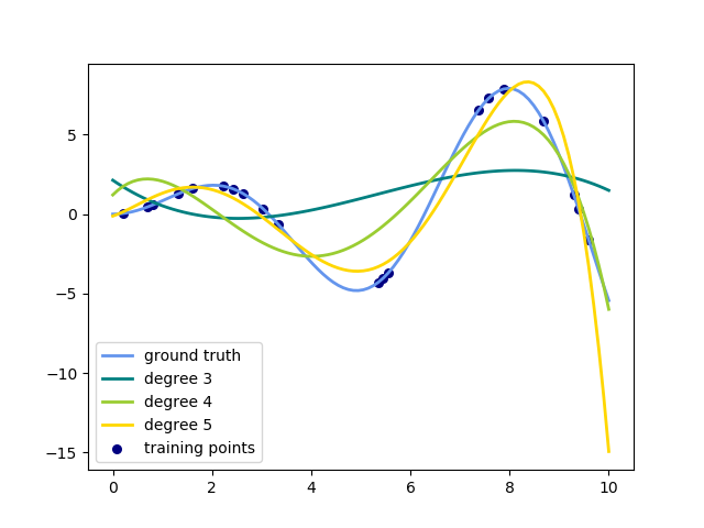
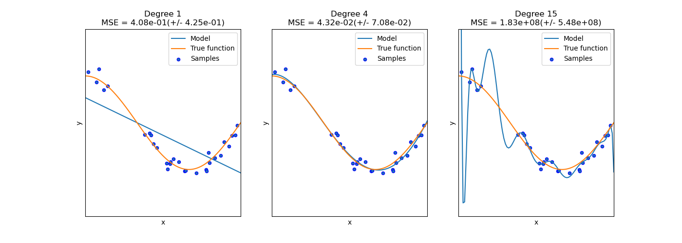
請注意,輸出數組中的要素數量與輸入數組的要素數量呈多項式比例關系,而度數呈指數關系。高度可能會導致過度擬合。
參見examples/linear_model/plot_polynomial_interpolation.py
示例
>>> import numpy as np
>>> from sklearn.preprocessing import PolynomialFeatures
>>> X = np.arange(6).reshape(3, 2)
>>> X
array([[0, 1],
       [2, 3],
       [4, 5]])
>>> poly = PolynomialFeatures(2)
>>> poly.fit_transform(X)
array([[ 1.,  0.,  1.,  0.,  0.,  1.],
       [ 1.,  2.,  3.,  4.,  6.,  9.],
       [ 1.,  4.,  5., 16., 20., 25.]])
>>> poly = PolynomialFeatures(interaction_only=True)
>>> poly.fit_transform(X)
array([[ 1.,  0.,  1.,  0.],
       [ 1.,  2.,  3.,  6.],
       [ 1.,  4.,  5., 20.]])
方法
| 方法 | 說明 |
|---|---|
fit(X[, y]) |
計算輸出要素的數量。 |
fit_transform(X[, y]) |
擬合數據,然后對其進行轉換。 |
get_feature_names([input_features]) |
返回輸出要素的要素名稱 |
get_params([deep]) |
獲取此估計量的參數。 |
set_params(**params) |
設置此估算器的參數。 |
transform(X) |
將數據轉換為多項式特征 |
__init__(degree=2, *, interaction_only=False, include_bias=True, order='C')
適合標簽編碼器
初始化self,有關準確的簽名,請參見help(type(self))。
fit(X, y=None)
計算輸出要素的數量。
| 參數 | 說明 |
|---|---|
| X | array-like, shape (n_samples, n_features) 數據。 |
| 返回值 | 說明 |
|---|---|
| self | instance |
fit_transform(X, y=None, **fit_params)
擬合數據,然后對其進行轉換。
使用可選參數fit_params將轉換器擬合到X和y,并返回X的轉換版本。
| 參數 | 說明 |
|---|---|
| X | {array-like, sparse matrix, dataframe} of shape (n_samples, n_features) |
| y | ndarray of shape (n_samples,), default=None 目標值。 |
| **fit_params | dict 其他擬合參數。 |
| 返回值 | 說明 |
|---|---|
| X_new | ndarray array of shape (n_samples, n_features_new) 轉換后的數組。 |
get_feature_names(input_features=None)
返回輸出要素的要素名稱
| 參數 | 說明 |
|---|---|
| input_features | list of string, length n_features, optional 輸入功能的字符串名稱(如果有)。默認情況下,使用“ x0”,“ x1”,……“ xn_features”。 |
| 返回值 | 說明 |
|---|---|
| output_feature_names | list of string, length n_output_features |
get_params(deep=True)
設置此估算器的參數。
該方法適用于簡單的估計器以及嵌套對象(例如管道)。后者的參數形式為<component>__<parameter>這樣就可以更新嵌套對象的每個組件。
| 參數 | 說明 |
|---|---|
| **params | dict 估算器參數。 |
| 返回值 | 說明 |
|---|---|
| self | object 估算器實例。 |
transform(X)
將數據轉換為多項式特征
| 參數 | 說明 |
|---|---|
| X | array-like or CSR/CSC sparse matrix, shape [n_samples, n_features] 數據要逐行轉換。 對于稀疏輸入(對于速度),CSR比CSC更可取,但如果度數為4或更高,則需要CSC。如果度數小于4,并且輸入格式為CSC,則將其轉換為CSR,生成多項式特征,然后轉換回CSC。 如果度為2或3,則使用Andrew Nystrom和John Hughes所描述的“利用稀疏度來使用K-Simplex數加快CSR矩陣的多項式特征展開”中描述的方法,它比在CSC輸入上使用的方法要快得多 。因此,CSC輸入將轉換為CSR,輸出將在返回之前轉換回CSC,因此優先選擇CSR。 |
| 返回值 | 說明 |
|---|---|
| XP | np.ndarray or CSR/CSC sparse matrix, shape [n_samples, NP] 特征矩陣,其中NP是從輸入組合生成的多項式特征的數量。 |