sklearn.linear_model.SGDClassifier?
class sklearn.linear_model.SGDClassifier(loss='hinge', *, penalty='l2', alpha=0.0001, l1_ratio=0.15, fit_intercept=True, max_iter=1000, tol=0.001, shuffle=True, verbose=0, epsilon=0.1, n_jobs=None, random_state=None, learning_rate='optimal', eta0=0.0, power_t=0.5, early_stopping=False, validation_fraction=0.1, n_iter_no_change=5, class_weight=None, warm_start=False, average=False)
具有SGD訓練的線性分類器(SVM,邏輯回歸等)。
該估計器通過隨機梯度下降(SGD)學習實現正則化線性模型:每次對每個樣本估計損失的梯度,并以遞減的強度(即學習率)沿此路徑更新模型。SGD允許通過該partial_fit方法進行小批量(在線/核心外)學習。為了使用默認學習率計劃獲得最佳結果,數據應具有零均值和單位方差。
此實現使用表示為密集或稀疏浮點值數組的數據。它所擬合的模型可以用損失參數來控制;默認情況下,它適用于線性支持向量機(SVM)。
正則化器是一個附加在損失函數上的懲罰,它使用平方歐氏范數L2或絕對范數L1或兩者的組合(彈性網)將模型參數收縮到零向量。如果由于正則化器的原因,參數更新跨越了0.0值,那么更新被截斷為0.0,以允許學習稀疏模型和實現在線特征選擇。
在用戶指南中閱讀更多內容。
| 參數 | 說明 |
|---|---|
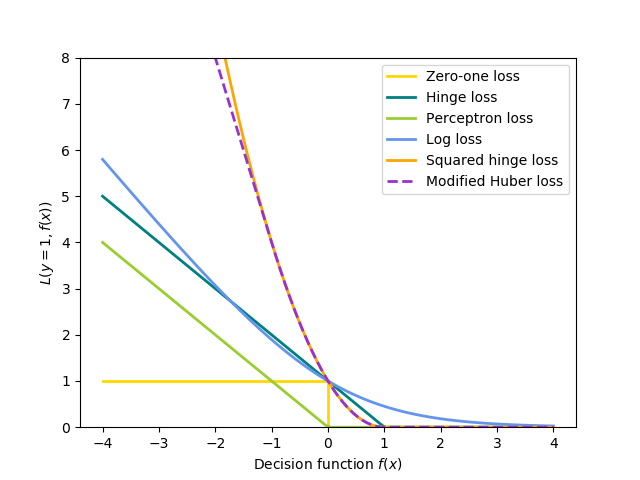
| loss | str, default=’hinge’ 要使用的損失函數。默認為'hinge',這將提供線性SVM。 可選項有“hinge”,“log”,“ modified_huber”,“ squared_hinge”,“ perceptron”或回歸損失:“ squared_loss”,“ huber”,“ epsilon_insensitive”或“ squared_epsilon_insensitive”。 log損失使邏輯回歸成為概率分類器。 'modified_huber'是另一個平滑的損失,它使異常值和概率估計具有一定的容忍度。“ squared_hinge”與hinge類似,但會受到二次懲罰。“perceptron”是感知器算法使用的線性損失。其他損失是為回歸而設計的,但也可用于分類。請參閱 SGDRegressor以獲取更多信息。 |
| penalty | {‘L2’, ‘L1’, ‘elasticnet’}, default=’L2’ 要使用的懲罰(又稱正則化)。默認值為“ L2”,這是線性SVM模型的標準正則化器。“ L1”和“ elasticnet”可能會給模型帶來稀疏性(特征選擇),而這是“ l2”無法實現的。 |
| alpha | float, default=0.0001 與正則項相乘的常數。值越高,正則化越強。當 learning_rate設置為“optimal” 時,也用于計算學習率。 |
| l1_ratio | float, default=0.15 彈性網混合參數,其中0 <= l1_ratio <=1。l1_ratio = 0對應于L2懲罰,l1_ratio = 1對應與L1懲罰。僅在 penalty為“ elasticnet”時使用。 |
| fit_intercept | bool, default=True 是否估計截距。如果為False,則假定數據已經中心化。 |
| max_iter | int, default=1000 通過訓練數據的最大次數(又稱歷元)。它只會影響 fit方法中的行為,而不會影響 partial_fit方法。0.19版本中的新功能。 |
| tol | float, default=1e-3 停止標準。如果不是None,則連續 n_iter_no_change次(eploss> best_loss-tol)時迭代將停止。0.19版本中的新功能。 |
| shuffle | bool, default=True 在每次迭代之后是否重新打亂訓練數據。 |
| verbose | int, default=0 日志的詳細程度。 |
| epsilon | float, default=0.1 僅當 loss是“ huber”,“ epsilon_insensitive”或“ squared_epsilon_insensitive”時,損失函數對epsilon是不敏感的。對于“huber”,確定一個閾值,在這個閾值上,準確預測變得不那么重要了。對于epsilon不敏感的情況,如果當前的預測和正確的標簽小于這個閾值,那么它們之間的任何差異都將被忽略。 |
| n_jobs | int, default=None 用于執行OVA(對于多類問題而言為“一個對所有”)的CPU內核數。除非 joblib.parallel_backend在上下文中進行了設置,否則None表示1 。 -1表示使用所有處理器。有關 更多詳細信息,請參見詞匯表。 |
| random_state | int, RandomState instance, default=None 用于打亂訓練數據,當 shuffle設置為 True。可以用一個整數為多個函數調用傳遞重復的輸出。請參閱詞匯表。 |
| learning_rate | str, default=’optimal’ 學習率參數: - ‘constant’: eta = eta0- ‘optimal’: eta = 1.0 / (alpha * (t + t0)),其中t0由Leon Bottou提出的啟發式方法選擇。- ‘invscaling’: eta = eta0 / pow(t, power_t)- ‘adaptive’:eta = eta0,只要訓練持續減少即可。如果early_stopping為True,每次迭代中連續n_iter_no_change次未能減少tol的訓練損失或未能增加tol的驗證分數,則當前學習率除以5。 *0.20版中的新功能:*添加了“adaptive”選項 |
| eta0 | double, default=0.0 “constant”,“invscaling”或“adaptive”,初始學習率。默認值為0.0,因為eta0沒有被默認的選項' optimal '。 |
| power_t | double, default=0.5 逆標度學習率指數[默認0.5]。 |
| early_stopping | bool, default=False 是否使用驗證提前停止終止訓練。如果設置為True,它將自動將訓練數據的分層部分的 score留作驗證,并在連續n_iter_no_change次的驗證分數沒有提高至少tol時終止訓練。0.20版中的新功能。 |
| validation_fraction | float, default=0.1 預留的訓練數據比例作為早期停止的驗證集。必須介于0和1之間。僅在 early_stopping為True時使用。 |
| n_iter_no_change | int, default=5 迭代次數,結果沒有改善,迭代需要提前停止。 *0.20版中的新功能:*添加了“ n_iter_no_change”選項 |
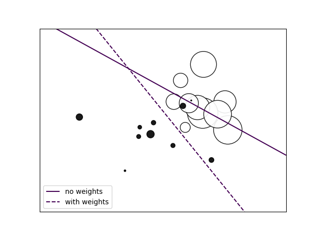
| class_weight | dict, {class_label: weight} or “balanced”, default=None 預設class_weight 擬合參數。 類別關聯的權重。如果沒有給出,所有類別的權重都應該是1。 “balanced”模式使用y的值來自動調整為與輸入數據中的類頻率成反比的權重。如 n_samples / (n_classes * np.bincount(y)) |
| warm_start | bool, default=False 設置為True時,重用前面調用的解決方案來進行初始化,否則,只清除前面的解決方案。請參閱詞匯表。 當warm_start為True時,重復調用fit或partial_fit可能會導致解決方案與一次調用fit時有所不同,這是因為數據的重排方式不同。如果使用動態學習率,則根據已經看到的樣本數調整學習率。調用 fit會重置此計數器,而partial_fit會導致增加現有計數器。 |
| average | bool or int, default=False 設置為True時,將計算平均SGD權重并將結果存儲在 coef_屬性中。如果將int設置為大于1,則一旦看到的樣本總數達到平均值就會開始平均。如average=10,將在看到10個樣本后開始平均。 |
| 屬性 | 說明 |
|---|---|
| coef_ | ndarray of shape (1, n_features) if n_classes == 2 else (n_classes, n_features) 分配給特征的權重。 |
| intercept_ | ndarray of shape (1,) if n_classes == 2 else (n_classes,) 決策函數中的常數項。 |
| n_iter_ | int 達到停止標準之前的實際迭代次數。對于多類別擬合,它是每個二分類擬合的最大值。 |
| loss_function_ | concrete LossFunction |
| classes_ | array of shape (n_classes,) |
| t_ | int 訓練期間進行的權重更新次數,與 (n_iter_ * n_samples)相同。 |
另見
線性支持向量分類。
邏輯回歸。
繼承自SGDClassifier。
Perceptron()等同于SGDClassifier(loss="perceptron", eta0=1, learning_rate="constant", penalty=None)。
示例
>>> import numpy as np
>>> from sklearn.linear_model import SGDClassifier
>>> from sklearn.preprocessing import StandardScaler
>>> from sklearn.pipeline import make_pipeline
>>> X = np.array([[-1, -1], [-2, -1], [1, 1], [2, 1]])
>>> Y = np.array([1, 1, 2, 2])
>>> # Always scale the input. The most convenient way is to use a pipeline.
>>> clf = make_pipeline(StandardScaler(),
...                     SGDClassifier(max_iter=1000, tol=1e-3))
>>> clf.fit(X, Y)
Pipeline(steps=[('standardscaler', StandardScaler()),
                ('sgdclassifier', SGDClassifier())])
>>> print(clf.predict([[-0.8, -1]]))
[1]
| 方法 | 說明 |
|---|---|
decision_function(self, X) |
預測樣本的置信度得分。 |
densify(self) |
將系數矩陣轉換為密集數組格式。 |
fit(self, X, y[, coef_init, intercept_init, …]) |
用隨機梯度下降擬合線性模型。 |
get_params(self[, deep]) |
獲取此估計器的參數。 |
partial_fit(self, X, y[, classes, sample_weight]) |
對給定的樣本進行一次隨機梯度下降。 |
predict(self, X) |
預測X中樣本的類別標簽。 |
score(self, X, y[, sample_weight]) |
返回給定測試數據和標簽上的平均準確度。 |
set_params(self, **kwargs) |
設置并驗證估計器的參數。 |
sparsify(self) |
將系數矩陣轉換為稀疏格式。 |
__init__(self, loss='hinge', *, penalty='l2', alpha=0.0001, l1_ratio=0.15, fit_intercept=True, max_iter=1000, tol=0.001, shuffle=True, verbose=0, epsilon=0.1, n_jobs=None, random_state=None, learning_rate='optimal', eta0=0.0, power_t=0.5, early_stopping=False, validation_fraction=0.1, n_iter_no_change=5, class_weight=None, warm_start=False, average=False)
初始化self, 請參閱help(type(self))以獲得準確的說明。
decision_function(self, X)
預測樣本的置信度得分。
樣本的置信度分數是該樣本到超平面的符號距離。
| 參數 | 說明 |
|---|---|
| X | array_like or sparse matrix, shape (n_samples, n_features) 樣本數據。 |
| 返回值 | 說明 |
|---|---|
| array, shape=(n_samples,) if n_classes == 2 else (n_samples, n_classes) 每個(樣本,類別)組合的置信度得分。在二分類情況下,self.classes_ [1]的置信度得分> 0表示將預測該類。 |
densify(self)
將系數矩陣轉換為密集數組格式。
將coef_數值(返回)轉換為numpy.ndarray。這是coef_的默認格式,并且是擬合模型所需的格式,因此僅在之前被稀疏化的模型上才需要調用此方法。否則,它是無操作的。
| 返回值 | 說明 |
|---|---|
| self | 擬合估計器。 |
fit(self, X, y, coef_init=None, intercept_init=None, sample_weight=None)
[源碼]
用隨機梯度下降擬合線性模型。
| 參數 | 說明 |
|---|---|
| X | {array-like, sparse matrix} of shape (n_samples, n_features) 訓練數據 |
| y | array-like of shape (n_samples,) 目標標簽。 |
| coef_init | ndarray of shape (n_classes, n_features), default=None 用于熱啟動優化的初始系數。 |
| intercept_init | ndarray of shape (n_classes,), default=None 初始截距以熱啟動優化。 |
| sample_weight | array-like, shape (n_samples,), default=None 權重應用于各個樣本。如果未提供,則假定權重相同。如果指定了class_weight,則這些權重將與class_weight(通過構造函數傳遞)相乘。 |
| 返回值 | 說明 |
|---|---|
| self | 返回self的實例。 |
get_params(self,deep = True )
[源碼]
獲取此估計器的參數。
| 參數 | 說明 |
|---|---|
| deep | bool, default=True 如果為True,返回此估計器和所包含子對象的參數。 |
| 返回值 | 說明 |
|---|---|
| params | mapping of string to any 參數名稱映射到其值。 |
partial_fit(self, X, y, classes=None, sample_weight=None)
[源碼]
對給定的樣本進行一次隨機梯度下降的迭代。
在內部,此方法使用max_iter = 1。因此,不能保證調用一次后達到損失函數的最小值。目標收斂、提前停止等問題由用戶自行處理。
| 參數 | 說明 |
|---|---|
| X | {array-like, sparse matrix}, shape (n_samples, n_features) 訓練數據的子集 |
| y | ndarray of shape (n_samples,) 目標值的子集 |
| classes | ndarray of shape (n_classes,), default=None partial_fit調用中所有的類。可以通過 np.unique(y_all)獲得,其中y_all是整個數據集的目標向量。第一次調用partial_fit時需要此參數,在后續調用中可以將其省略。請注意,y不需要包含classes中的所有標簽。 |
| sample_weight | array-like, shape (n_samples,), default=None 權重應用于各個樣本。如果未提供,則假定權重相同。 |
| 返回值 | 說明 |
|---|---|
| self | 返回self的實例。 |
predict(self, X)
[源碼]
預測X中樣本的類別標簽。
| 參數 | 說明 |
|---|---|
| X | array_like or sparse matrix, shape (n_samples, n_features) 樣本數據 |
| 返回值 | 說明 |
|---|---|
| C | array, shape [n_samples] 每個樣本的預測類別標簽。 |
property predict_log_proba
概率估計的對數。
此方法僅適用于對數損失和修正Huber損失。
當loss =“ modified_huber”時,概率估計只可能是0和1,所以取對數是不可能的。
詳細信息請參見predict_proba。
| 參數 | 說明 |
|---|---|
| X | {array-like, sparse matrix} of shape (n_samples, n_features) 進行預測的樣本數據。 |
| 返回值 | 說明 |
|---|---|
| T | array-like, shape (n_samples, n_classes) 返回模型中每個類的樣本的對數概率,按 self.classes_中的類別順序排序 。 |
property predict_proba
概率估計。
此方法僅適用于對數損失和修正Huber損失。
根據Zadrozny和Elkan的建議,通過簡單的歸一化方法從二元(one-vs.-rest)估計值中得出多類概率估計值。
對于損失函數為“ modified_huber”的二分類概率估計值由(clip(decision_function(X),-1,1)+ 1)/ 2給出。對于其他損失函數,有必要通過用sklearn.calibration.CalibratedClassifierCV分類器包裹來進行適當的概率校準 。
| 參數 | 說明 |
|---|---|
| X | {array-like, sparse matrix}, shape (n_samples, n_features) 進行預測的樣本數據。 |
| 返回值 |
|---|
| ndarray of shape (n_samples, n_classes) 返回模型中每個類的樣本概率,按 self.classes_中的類別順序排序 。 |
參考
Zadrozny and Elkan, “Transforming classifier scores into multiclass probability estimates”, SIGKDD’02, http://www.research.ibm.com/people/z/zadrozny/kdd2002-Transf.pdf
The justification for the formula in the loss=”modified_huber” case is in the appendix B in: http://jmlr.csail.mit.edu/papers/volume2/zhang02c/zhang02c.pdf
score(self,X,y,sample_weight = None )
[源碼]
返回給定測試數據和標簽上的平均準確度。
在多標簽分類中,這是子集準確性,這是一個嚴格的指標,因為你需要為每個樣本正確預測對應的標簽集。
| 參數 | 說明 |
|---|---|
| X | array-like of shape (n_samples, n_features) 測試樣本。 |
| y | array-like of shape (n_samples,) or (n_samples, n_outputs) X的真實標簽。 |
| sample_weight | array-like of shape (n_samples,), default=None 樣本權重。 |
| 返回值 | 說明 |
|---|---|
| score | float 預測標簽與真實標簽的平均準確度 |
set_params(self, **kwargs)
[源碼]
設置并驗證估計器的參數。
| 參數 | 說明 |
|---|---|
| **kwargs | dict 估計器參數。 |
| 返回值 | 說明 |
|---|---|
| self | object 估計器實例。 |
sparsify(self)
[源碼]
將系數矩陣轉換為稀疏格式。
將coef_數值轉換為scipy.sparse矩陣,對于L1正規化的模型,該矩陣比通常的numpy.ndarray具有更高的內存和存儲效率。
該intercept_數值未轉換。
| 返回值 | 說明 |
|---|---|
| self | 擬合估計器。 |
注
對于非稀疏模型,即當coef_中零的個數不多時,這實際上可能會增加內存使用量,因此請謹慎使用此方法。經驗法則是,可以使用(coef_ == 0).sum()計算得到的零元素的數量必須大于50%,這時的效果是顯著的。
在調用densify之前,調用此方法將無法進一步使用partial_fit方法(如果有)。