scikit-learn 0.22中的發布要點?

我們很高興地宣布發布scikit-learn 0.22，這里許多bug被修復和一些新的功能！我們在下面詳細介紹了這個版本的幾個主要特性。有關所有更改的詳盡清單，請參閱發布說明。

若要安裝最新版本(使用 pip)，請執行以下操作：

pip install --upgrade scikit-learn

或者使用conda安裝：

conda install scikit-learn

1.2.1 新的繪圖API

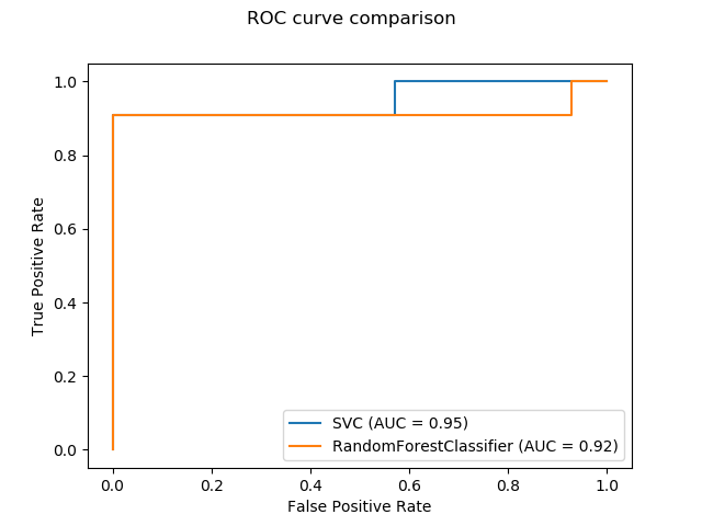
一個新的繪圖API可用于創建可視化。這個新的API允許快速調整一個情節的視覺，而不涉及任何恢復。還可以在同一畫布上添加不同的圖。下面的示例說明了 plot_roc_curve，但也支持其他繪圖實用程序， plot_partial_dependence,plot_precision_recall_curve, and plot_confusion_matrix.。在用戶指南中閱讀有關此新API的更多信息。

from sklearn.model_selection import train_test_split
from sklearn.svm import SVC
from sklearn.metrics import plot_roc_curve
from sklearn.ensemble import RandomForestClassifier
from sklearn.datasets import make_classification
import matplotlib.pyplot as plt

X, y = make_classification(random_state=0)
X_train, X_test, y_train, y_test = train_test_split(X, y, random_state=42)

svc = SVC(random_state=42)
svc.fit(X_train, y_train)
rfc = RandomForestClassifier(random_state=42)
rfc.fit(X_train, y_train)

svc_disp = plot_roc_curve(svc, X_test, y_test)
rfc_disp = plot_roc_curve(rfc, X_test, y_test, ax=svc_disp.ax_)
rfc_disp.figure_.suptitle("ROC curve comparison")

plt.show()

1.2.2 Stacking 分類器和回歸器

StackingClassifier 和 StackingRegressor 允許您有一堆帶有最終分類器或回歸器的估計器。疊加泛化是將單個估計器的輸出疊加起來，并使用分類器來計算最終的預測。Stacking允許使用每個單獨的估計器的強度，使用它們的輸出作為最終估計器的輸入。基估計器是在全X上擬合的，而最終估計器是使用 cross_val_predict對基估計器進行交叉驗證的預測來訓練的。

在用戶指南中閱讀更多內容。

from sklearn.datasets import load_iris
from sklearn.svm import LinearSVC
from sklearn.linear_model import LogisticRegression
from sklearn.preprocessing import StandardScaler
from sklearn.pipeline import make_pipeline
from sklearn.ensemble import StackingClassifier
from sklearn.model_selection import train_test_split

X, y = load_iris(return_X_y=True)
estimators = [
    ('rf', RandomForestClassifier(n_estimators=10, random_state=42)),
    ('svr', make_pipeline(StandardScaler(),
                          LinearSVC(random_state=42)))
]
clf = StackingClassifier(
    estimators=estimators, final_estimator=LogisticRegression()
)
X_train, X_test, y_train, y_test = train_test_split(
    X, y, stratify=y, random_state=42
)
clf.fit(X_train, y_train).score(X_test, y_test)

# 輸出
0.9473684210526315

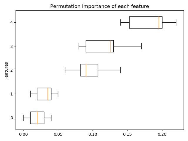
1.2.3 基于置換的特征重要性

為了得到每個特征的重要性，可以使用 inspection.permutation_importance，對于任何合適的估計器：

from sklearn.ensemble import RandomForestClassifier
from sklearn.inspection import permutation_importance

X, y = make_classification(random_state=0, n_features=5, n_informative=3)
rf = RandomForestClassifier(random_state=0).fit(X, y)
result = permutation_importance(rf, X, y, n_repeats=10, random_state=0,
                                n_jobs=-1)

fig, ax = plt.subplots()
sorted_idx = result.importances_mean.argsort()
ax.boxplot(result.importances[sorted_idx].T,
           vert=False, labels=range(X.shape[1]))
ax.set_title("Permutation Importance of each feature")
ax.set_ylabel("Features")
fig.tight_layout()
plt.show()

1.2.4 梯度提升的原生缺失值支持

ensemble.HistGradientBoostingClassifier 和 ensemble.HistGradientBoostingRegressor現在有了對缺失值(NaNs)的原生支持。這意味著在訓練或預測時不需要計算數據。

from sklearn.experimental import enable_hist_gradient_boosting  # noqa
from sklearn.ensemble import HistGradientBoostingClassifier
import numpy as np

X = np.array([0, 1, 2, np.nan]).reshape(-1, 1)
y = [0, 0, 1, 1]

gbdt = HistGradientBoostingClassifier(min_samples_leaf=1).fit(X, y)
print(gbdt.predict(X))

# 輸出
[0 0 1 1]

1.2.5 預計算稀疏近鄰圖

現在大多數基于最近鄰圖的估計器都接受預先計算的稀疏圖作為輸入，以重用相同的圖以滿足多個估計器的訓練。要在管道中使用此特性，可以使用memory參數，以及兩個新的轉換器之一， neighbors.KNeighborsTransformer 和 neighbors.RadiusNeighborsTransformer。預計算還可以由自定義估計器執行，以使用替代實現，例如近似最近鄰方法。請參閱用戶指南中的詳細信息。

from tempfile import TemporaryDirectory
from sklearn.neighbors import KNeighborsTransformer
from sklearn.manifold import Isomap
from sklearn.pipeline import make_pipeline

X, y = make_classification(random_state=0)

with TemporaryDirectory(prefix="sklearn_cache_") as tmpdir:
    estimator = make_pipeline(
        KNeighborsTransformer(n_neighbors=10, mode='distance'),
        Isomap(n_neighbors=10, metric='precomputed'),
        memory=tmpdir)
    estimator.fit(X)

    # We can decrease the number of neighbors and the graph will not be
    # recomputed.
    estimator.set_params(isomap__n_neighbors=5)
    estimator.fit(X)

1.2.6 基于KNN的估算

我們現在支持使用k近鄰來完成缺失值的估算。

每個樣本的缺失值都是使用訓練集中最近的 n_neighbors個最近鄰居的平均值來估算的。如果兩個都不缺少的特征接近，則兩個樣本是接近的。默認情況下，歐氏距離度量支持缺失值的， nan_euclidean_distances距離用于查找最近的鄰居。

在用戶指南中閱讀更多內容。

import numpy as np
from sklearn.impute import KNNImputer

X = [[1, 2, np.nan], [3, 4, 3], [np.nan, 6, 5], [8, 8, 7]]
imputer = KNNImputer(n_neighbors=2)
print(imputer.fit_transform(X))

# 輸出
[[1.  2.  4. ]
 [3.  4.  3. ]
 [5.5 6.  5. ]
 [8.  8.  7. ]]

1.2.7 樹剪枝

現在，一旦樹木建成，就可以修剪大多數基于樹的估計器了。剪枝是基于最小的成本復雜度。有關詳細信息，請參閱用戶指南中的更多內容。

X, y = make_classification(random_state=0)

rf = RandomForestClassifier(random_state=0, ccp_alpha=0).fit(X, y)
print("Average number of nodes without pruning {:.1f}".format(
    np.mean([e.tree_.node_count for e in rf.estimators_])))

rf = RandomForestClassifier(random_state=0, ccp_alpha=0.05).fit(X, y)
print("Average number of nodes with pruning {:.1f}".format(
    np.mean([e.tree_.node_count for e in rf.estimators_])))

# 輸出
Average number of nodes without pruning 22.3
Average number of nodes with pruning 6.4

1.2.8 從OpenML檢索數據

datasets.fetch_openml現在可以返回pandas數據，從而正確處理異構數據集：

from sklearn.datasets import fetch_openml

titanic = fetch_openml('titanic', version=1, as_frame=True)
print(titanic.data.head()[['pclass', 'embarked']])

# 輸出
   pclass embarked
0     1.0        S
1     1.0        S
2     1.0        S
3     1.0        S
4     1.0        S

1.2.9 檢驗scikit-learn估計器的兼容性

開發人員可以使用check_estimator檢查他們的scikit-learn兼容估計器的兼容性。例如，通過check_estimator(LinearSVC)。

我們現在提供了一個pytest 特定的裝飾器，它允許pytest獨立運行所有檢查并報告失敗的檢查。

from sklearn.linear_model import LogisticRegression
from sklearn.tree import DecisionTreeRegressor
from sklearn.utils.estimator_checks import parametrize_with_checks


@parametrize_with_checks([LogisticRegression, DecisionTreeRegressor])
def test_sklearn_compatible_estimator(estimator, check):
    check(estimator)
  
# 輸出
/home/circleci/project/sklearn/utils/estimator_checks.py:420: FutureWarning: Passing a class is deprecated since version 0.23 and won't be supported in 0.24.Please pass an instance instead.
  warnings.warn(msg, FutureWarning)

1.2.10 ROC AUC 現在支持多類分類

roc_auc_score函數也可用于多類分類。目前支持兩種平均策略：one-vs-one算法計算成對的ROC AUC分數的平均值，one-vs-rest算法計算每一類相對于所有其他類的平均分數。在這兩種情況下，多類ROC AUC分數是根據該模型從樣本屬于特定類別的概率估計來計算的。OvO和OvR算法均支持相同加權(average='macro')和根據流行程度的加權(average='weighted')。

在用戶指南中閱讀更多內容。

from sklearn.datasets import make_classification
from sklearn.svm import SVC
from sklearn.metrics import roc_auc_score

X, y = make_classification(n_classes=4, n_informative=16)
clf = SVC(decision_function_shape='ovo', probability=True).fit(X, y)
print(roc_auc_score(y, clf.predict_proba(X), multi_class='ovo'))

# 輸出
0.9984000000000001

腳本的總運行時間：(0分4.999秒)